Stanford AA203 Optimal and Learning‑Based Control ｜ Spring 2026 ｜ Lecture 3： Calculus of Variations — Annotated Lecture Notes & Key Takeaways

Course Information

Institution: Stanford

Original Course: Stanford AA203 Optimal and Learning‑Based Control ｜ Spring 2026 ｜ Lecture 3： Calculus of Variations

Instructor Bio: Delivered by Prof. Marco Pavone and Dr. Daniele Gammelli. Their research spans the mathematical foundations of optimal control and robotic system implementation.

Course Description: This session focuses on the calculus of variations, a classical optimal control tool. It covers problem formulation, Euler-Lagrange equation derivation and boundary conditions, and methods for solving functional extrema in continuous systems.

These notes cover Lecture 3 of Stanford's AA203 course, focused on calculus of variations. The session opens with a quick instructor introduction, then jumps into reviewing prior optimal control material before unpacking inequality-constrained optimization, active constraints, and the path toward KKT optimality conditions. I tried to capture both what the presenter laid out and the confusing spots from in-lecture student back-and-forth.
 

Recap of prior optimal control setup

 

The instructor opens by orienting everyone to the day's agenda. He touches on material from the previous week, where the class built the high-level formulation for optimal control problems.
 

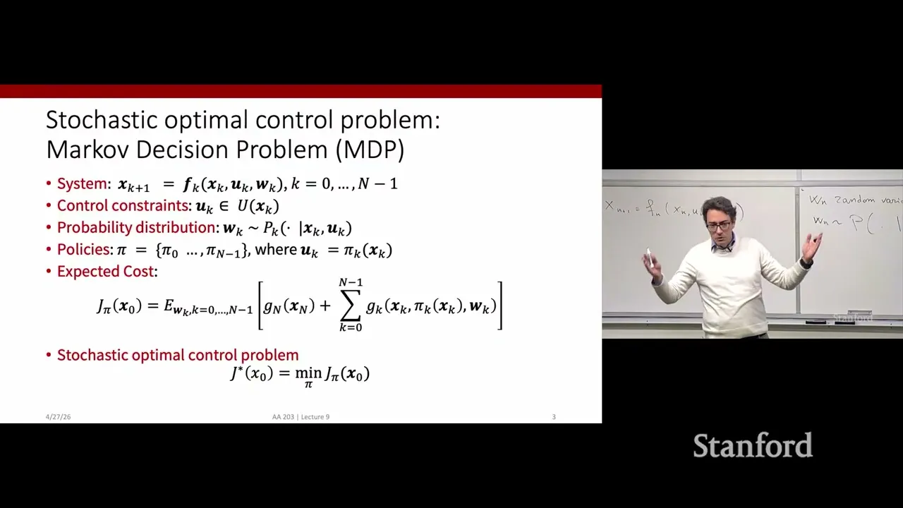
We start with a dynamical system described by differential equations, with state trajectory x(t)x(t). The job is to find an optimal control signal u∗(t)u∗(t) that minimizes an objective functional. That objective functional J has two distinct pieces: a terminal cost h(x(tf))h(x(tf​)), evaluated at the final time tftf​, and a running cost that accumulates across the whole time horizon.
 

He flags that this kind of optimal control problem lives in an infinite-dimensional space. Unlike finite-dimensional problems where you optimize over a fixed set of real numbers, here we optimize over entire functions of time. That distinction matters because the math rules we use for finite dimensions cannot always be carried over directly.
 

Before diving into calculus of variations proper, the lecture pauses to wrap up finite-dimensional constrained optimization. Last week covered unconstrained optimization, where a necessary condition for minima is that the gradient of the objective equals zero — a stationary point. They also worked through equality-constrained optimization. Today's session finishes the finite-dimensional material with inequality constraints, then shifts to building optimality conditions for the infinite-dimensional optimal control setting.
 

Inequality-constrained problems and active-constraint reasoning

 

The core of this segment works through the inequality-constrained problem, shortened in the lecture as ICP. We minimize an objective function f(x)f(x), subject to a mix of equality constraints hi(x)=0hi​(x)=0 and inequality constraints gj(x)≤0gj​(x)≤0. Every function f, hihi​, gjgj​ is assumed continuously differentiable.
 

A critical definition gets introduced here: active versus inactive inequality constraints. At a feasible point x, an inequality constraint counts as active when gj(x)=0gj​(x)=0. The constraint sits right on its boundary. If gj(x)<0gj​(x)<0, that constraint is inactive — there's slack, and we're safely inside the allowed region.
 

The instructor walks through a simple visual example: minimize x+yx+y, subject to x≥0x≥0, y≥0y≥0, x+y≤3x+y≤3. At the origin (0,0)(0,0), the two non-negativity constraints hit equality (active), and x+y≤3x+y≤3 holds with slack (inactive).
 

He lays out a central claim: if x is a local minimum for the full inequality-constrained problem, then x is also a local minimum for a modified problem where we drop all inactive constraints and keep only the active ones.
 

The supporting argument uses proof-by-contradiction logic (07:58). Suppose x is a local minimum for the full problem, but not a local minimum once inactive constraints are removed. If that were true, we could move a tiny bit within a small neighborhood around x, still respecting the remaining active and equality constraints, and find another point with a smaller objective value.
 

Since inactive constraints hold strictly less than zero at x, we can shrink the neighborhood small enough that those inactive constraints remain satisfied everywhere inside it. If we can find a better point in that neighborhood, that same point would also satisfy every constraint of the original full problem. That directly contradicts the premise that x was a local minimum for the full problem. So the supposition must be wrong.
 

One point that was hard to follow here is how boundary status interacts with this claim. A student pushes on exactly this nuance. If we sit right on a constraint boundary, outside the feasible region there might exist points with even lower objective values — but those points violate constraints and don't count. The theorem only talks about feasible points inside the tiny neighborhood. The lecturer emphasizes this is a sketched intuitive argument rather than a fully rigorous formal proof.
 

This trick of discarding inactive constraints is described as the "easy route." Instead of building theory for inequality constraints from scratch, we convert active inequalities into effective equality constraints, so we can reuse all the math already built for equality-constrained optimization.
 

Moving toward KKT conditions and Lagrange multipliers

 

Now that we know active inequalities can be treated like equalities at a local minimum, Lagrange multipliers come back from the equality-constrained case.
 

For pure equality constraints, we build a Lagrangian L(x,λ)L(x,λ) by taking the objective function and adding weighted copies of each equality constraint, with weights λiλi​ as the Lagrange multipliers. A necessary optimality condition says the gradient of this Lagrangian with respect to x must equal zero. This gives a system of equations with n+mn+m unknowns to solve.
 

For inequality-constrained problems, we extend this setup. We add multipliers μjμj​ for each inequality constraint. Inactive constraints get μj=0μj​=0, so they contribute nothing to the Lagrangian sum. Active constraints have non-zero multipliers. There's one extra rule: multipliers linked to inequality constraints must be non-negative.
 

Taken together, these rules form the Karush-Kuhn-Tucker (KKT) conditions. The lecturer notes he'll skip deep geometric interpretation and formal proof for the sign requirement on multipliers, since it falls outside this lecture's scope.
 

A student poses a practical question. If we solve the reduced problem using only active constraints, can we automatically trust that all inactive constraints will hold? Or do we need to iterate and check?
 

The instructor clarifies what the theorem actually delivers. The statement is a necessary condition. If x is a local minimum of the original problem, then x must also be a local minimum of the problem stripped of inactive constraints. It does not work in the other direction. Solving the reduced problem does not guarantee the solution will satisfy the previously-inactive constraints. In practice, you'd need to check feasibility after solving, and potentially iterate if constraints switch between active and inactive.
 

The lecturer walks back to the two-variable example to illustrate notation. In that example there are no equality constraints hihi​, only three inequality constraints g1,g2,g3g1​,g2​,g3​. He notes the problem statement uses gj(x)≤0gj​(x)≤0, so inequalities written with ≥≥ need a sign flip to fit the standard form. The set A(x)A(x) is the collection of active constraints, and this set changes depending on which feasible point x you evaluate it at.
 

Unanswered and under-explored points

 

Several ideas get mentioned without full resolution during this segment.
 

First, the whole active-constraint argument is presented as an intuitive sketch, not a rigorous proof. Multiple times the instructor says listeners shouldn't treat it as perfectly air-tight formal mathematics. There are edge-case assumptions like constraint qualification that never get unpacked. Constraint qualifications matter because KKT conditions can break down without them, but that topic gets deferred.
 

Second, we only cover necessary optimality conditions. There's no discussion of sufficient conditions that would let us confirm a candidate point truly is a minimum. We know what properties any local minimum must satisfy, but satisfying KKT doesn't guarantee you have one.
 

Third, the practical algorithm side gets almost no attention. We learn the theoretical conditions, but there's no walk-through of how you would computationally identify active constraint sets in real-world numerical solvers. Students ask about iteration, but only get a high-level conceptual remark.
 

The lecture wraps this finite-dimensional optimization block by stating that all this groundwork sets up the main target: deriving analogous necessary optimality conditions for the infinite-dimensional optimal control problem — which is where calculus of variations comes into play.

Content Disclaimer: This article is for general reference only and does not constitute professional R&D guidance, production process advice or quality certification. All material performance data has specific test premises; readers should verify parameters against actual equipment and working conditions.