Stanford AA203 Optimal and Learning-Based Control | Spring 2026 | Lecture 1: Course Overview — Annotated Lecture Notes & Key Takeaways

Course Information

Institution: Stanford

Original Course: Stanford AA203 Optimal and Learning-Based Control | Spring 2026 | Lecture 1: Course Overview

Instructor Bio: Delivered by Prof. Marco Pavone and Dr. Daniele Gammelli from Stanford’s Autonomous Systems Lab (ASL). Prof. Pavone specializes in optimal control and autonomous systems; Dr. Gammelli focuses on reinforcement learning for control engineering.

Course Description: This opening session outlines the course structure, learning objectives and assessment scheme. It introduces real-world use cases of optimal and learning-based control, previews foundational nonlinear optimization, and presents course tools and resources.

If you missed the first lecture of AA203, these notes walk you through everything Marco Pavone covered — from syllabus logistics to the big-picture motivation for studying optimal and learning-based control. This class sits at the intersection of robotics, control theory, and machine learning, and Pavone frames it as a broad survey rather than a deep dive into any single method.
 

Course Logistics, Grading, and What You’ll Actually Need

 

The instructor is Marco Pavone, a professor in Aeronautics and Astronautics with additional appointments in computer science and electrical engineering. He runs Stanford’s Autonomous Systems Lab and also leads autonomous systems research at Nvidia, so he brings both academic and industry perspective to the material.
 

Grading is straightforward, if heavily weighted toward homework. There are four graded problem sets, each worth 20% of your final grade, for a total of 80%. The final exam on June 8 (3:30–6:30 PM) makes up the remaining 20%. You can also earn up to 5% bonus credit for meaningful participation on Ed — answering classmates’ questions thoughtfully, not just posting short comments.
 

Homework will be released on Fridays and due on Fridays, spaced roughly evenly through the quarter. Each assignment mixes theoretical derivation problems and Python coding exercises.
 

The late policy is generous but requires strategy. You get six total free late days to use across all assignments, but you can apply at most two to any single problem set. Pavone advised being intentional about how you spend them, since unexpected things always come up over the quarter.
 

For the first four weeks, there are optional Friday recitations from 1:30 to 2:30 PM. They cover foundational tools you’ll need later in the class, like Jax and basic regression models. You don’t have to attend if you’re already comfortable with those topics, and all sessions will be recorded.
 

All core materials — lecture slides, official course notes, and the full syllabus — are posted on the course website. There’s also a list of optional textbooks and references if you want to dig deeper into specific topics, but none are required to follow along or do the homework.
 

Prerequisites, Self-Assessment, and How Hard This Class Actually Is

 

Pavone was clear about what background you absolutely need, and what you can get away with not knowing.
 

You must be comfortable with multivariable calculus, vector calculus, and ordinary differential equations. You don’t need to be an expert at solving complicated ODEs analytically, but you need to understand what they represent and how they work. Linear algebra is also non-negotiable.
 

Prior exposure to optimization, machine learning, or classical control is helpful but not required. The class is designed to be self-contained, but having that background will make the material land much faster.
 

To help you gauge whether you’re ready, there’s an ungraded “homework zero” already posted online, with solutions provided. Pavone explicitly told students not to use ChatGPT on it. The point is not to get a perfect score — it’s to test your own knowledge and see which areas feel rusty. If you find the problems extremely difficult, he suggested taking relevant prerequisite courses first and coming back to AA203 later. If you’re just shaky in a few spots, you can brush up as the quarter goes on.
 

Overall, he called the class “quite challenging” but not extreme. The breadth of topics means you’ll be stretched across calculus, statistics, and coding all at once, rather than going deep in any single area.
 

What Classical Control Misses — and Why We Need Optimal and Learning-Based Control

 

Pavone spent a good chunk of the lecture building up why this class exists, starting from the most basic idea of what a control system even is.
 

At its simplest, a control system has a system — physical, financial, or digital — sensors that measure its state, a controller that decides what action to take, and actuators that carry out that action. The whole thing runs in a loop: measure the state, compute a control input, apply it, watch the response, and repeat. He used relatable examples — a human walking toward a door, a thermostat heating a house, a car staying in its lane — to make the point that everyone intuitively performs closed-loop control every day.
 

Classical control methods like PID handle the basics well. They keep systems stable, let you track a reference signal, reject outside disturbances like wind gusts, and work even if your system model is slightly wrong. But Pavone argued there are three big gaps that classical control doesn’t really address.
 

First, it says nothing about optimality. There are lots of ways to stabilize a system, but which one uses the least control effort? Which one gets the job done fastest? Classical control has no answer for that.
 

Second, it takes the reference signal as a given. Where does the desired trajectory actually come from in the first place? That’s the planning problem, and it’s inseparable from control if you’re building something like an autonomous aircraft.
 

Third, classical control assumes you already have a working model of the system. What if you don’t? Or what if the system changes over time as it wears down or operates in new conditions? That’s where learning from data becomes necessary.
 

Those three gaps — optimality, planning, and adaptation through learning — are exactly what optimal and learning-based control is built to address.
 

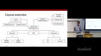
How the Course Is Structured: From Open-Loop to Learning-Based Methods

 

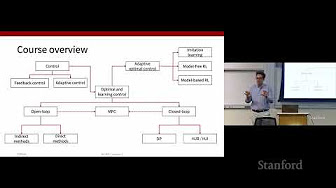
The course splits roughly into two halves. The first half assumes you have an approximate model of the system. The second half drops that assumption entirely and works directly with data.
 

Open-loop optimal control

 

We start with open-loop methods. In open-loop control, you compute an entire sequence of actions ahead of time and then execute them blindly, with no new feedback along the way. Pavone used the silly but memorable example of closing your eyes and walking toward a door — you plan your path ahead of time and hope nobody steps in front of you.
 

It sounds strictly worse than closed-loop, and in terms of robustness it is. But it’s computationally extremely efficient, which makes it very useful in practice. There are two main families of methods: indirect and direct. We’ll spend the first two to three weeks on this material.
 

Closed-loop optimal control

 

Closed-loop methods use feedback and re-plan as you go. They’re much more powerful at handling disturbances and uncertainty, but computationally far heavier, because you have to account for every possible future situation that might arise.
 

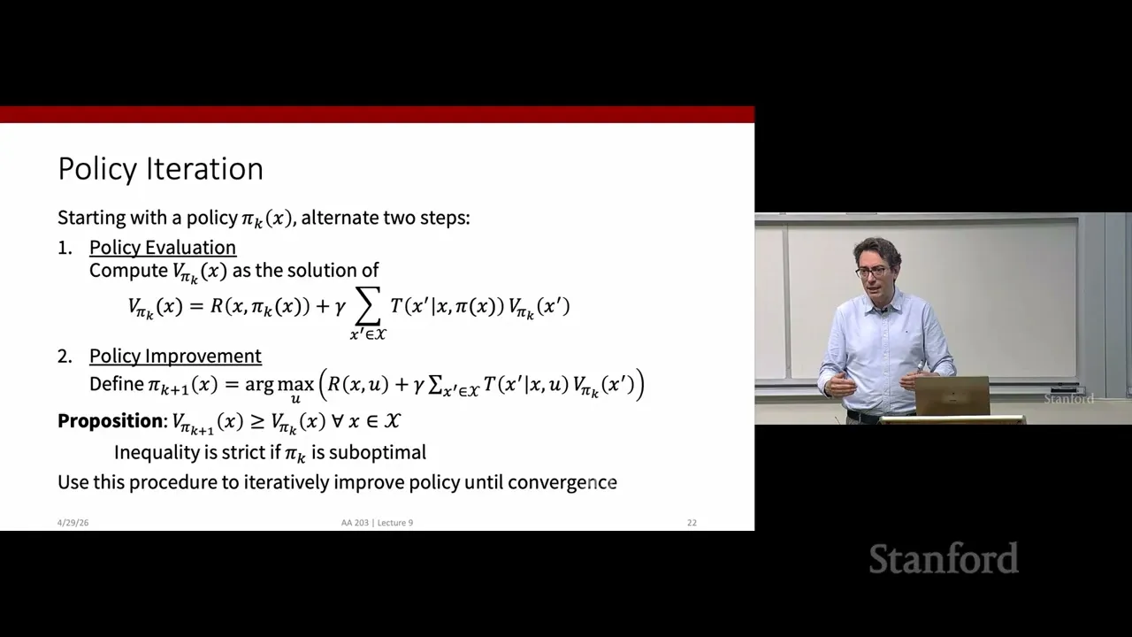
This is where dynamic programming lives, along with the Hamilton-Jacobi-Bellman and Hamilton-Jacobi-Isaacs equations. These are continuous-time versions of dynamic programming ideas you might have seen in decision-making classes. They’re also useful for building formal safety guarantees around controllers. We’ll spend about two weeks on this material.
 

Model predictive control (MPC)

 

MPC is the bridge between open and closed loop, and Pavone called it the second most widely used control methodology in industry after PID.
 

The core idea is simple: at every time step, you solve an open-loop optimal control problem, execute just the first action in the sequence, then take a new measurement and solve the whole thing again. You get the feedback benefits of closed loop, but you only ever solve one open-loop problem at a time. We’ll cover MPC over about two to three lectures.
 

Learning-based control

 

In the second half of the course, we stop assuming we have a good model and instead learn controller behavior directly from data. Pavone walked through three broad approaches.
 

Imitation learning is the first: you watch an expert demonstrate the right behavior, then train a policy to copy it. It’s a good way to bootstrap a working controller quickly.
 

Reinforcement learning is the second: instead of copying an expert, the agent learns by trial and error, using a reward signal to improve over time. It comes in model-based and model-free flavors.
 

Pavone emphasized that these aren’t competing approaches. In practice, people almost always mix them. For autonomous driving, for example, you’d typically use imitation learning to get a decent initial policy, then refine it with reinforcement learning. The same is true for modern autonomy stacks more broadly — supervised fine-tuning first, then RL improvement.
 

One point that was hard to follow at first is why we spend so much time on classical optimal control if learning-based methods are so hyped right now. Pavone’s answer was that in real robotic systems, you use all of these tools. You can’t just throw a model-free RL algorithm at every problem and expect it to work. Knowing when to use each tool is the real skill, and that’s what the class aims to teach.
 

The Three Ingredients of an Optimal Control Problem

 

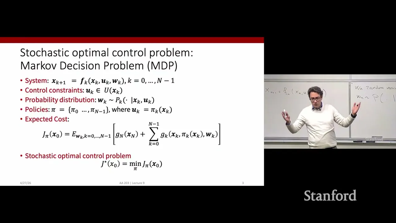
Toward the end of the lecture, Pavone broke down what actually defines an optimal control problem. There are three essential pieces.
 

First is a mathematical model of the system. For this class, that means a system of ordinary differential equations. Pavone gave a very pragmatic interpretation of ODEs: they’re just a mechanism for predicting the future state of the system, given its current state and the control inputs you apply.
 

He walked through the intuition step by step. The derivative of state tells you how fast the state is changing. Multiply by a small time step, and you can approximate what the state will be a moment from now. That’s the core idea — no fancy math magic, just a prediction rule.
 

The class uses standard vector notation: bold x for the state vector and bold u for the control input vector. The function f maps state and control to the state derivative. Importantly, f can also depend explicitly on time, meaning the system might behave differently at different times even with the exact same state and input.
 

He also defined a few terms we’ll use all quarter: a control history is the full sequence of control inputs over time, and a trajectory is the corresponding sequence of states over the interval from initial time t₀ to final time tբ.
 

Second are constraints. These are hard limits like “don’t hit the other car” in autonomous driving. Classical control rarely handles constraints explicitly, but optimal control builds them right into the problem formulation from the start.
 

Third is a performance criterion, also called a cost function or performance index. This is where you encode what you care about: tracking error, control effort, time to reach the goal, or some weighted combination. Usually these goals conflict — going faster almost always uses more energy, for example. The performance index lets you formally trade them off against each other.
 

Pavone ended this section right as class hit the mid-lecture break, so we didn’t get into actual cost function math yet. That’s coming up next lecture.
 

Open Thoughts and What to Watch For

 

A few things stood out as either unclear or worth flagging as you start the class.
 

First, the breadth-over-depth tradeoff is very real. Pavone explicitly said the class prioritizes wide exposure over deep mastery, so if you want to truly master any single method, you’ll need to do extra reading on your own. That’s not a flaw — it’s a deliberate design choice — but it’s good to know going in.
 

Second, the line between “optimal control” and “learning-based control” can feel blurry at first. A lot of learning-based control is still optimal control, just with a learned model instead of a hand-derived one. The class treats them as two halves of the same bigger picture, which is a useful framing once it clicks.
 

Finally, Pavone mentioned that all the methods in the class are really solving the same underlying problem, just with different assumptions. That’s a useful north star to keep in mind as we move through very different-looking techniques over the quarter.
 

By the end of the first lecture, you get a clear sense of what AA203 is about: a wide-ranging tour of optimal and learning-based control, with equal parts theory and Python implementation, focused on giving you the toolkit to pick the right method for the right problem. If you work through homework zero and brush up on any rusty linear algebra or ODE skills, you should be in good shape for the rest of the quarter.

 

Reference Block:

 

Source Reference Link: Not provided Link Brief: Based on the Spring 2026 first lecture transcript of Stanford AA203, these notes summarize course logistics, prerequisites, structure, and core control concepts for students who missed class.
 

Content Disclaimer:

 

This article is for general reference only and does not constitute professional R&D guidance, production process advice or quality certification. All material performance data has specific test premises; readers should verify parameters against actual equipment and working conditions.