Stanford AA203 Optimal and Learning‑Based Control ｜ Spring 2026 ｜ Lecture 7： Dynamic Programming— Annotated Lecture Notes & Key Takeaways

Course Information

Institution: Stanford

Original Course: Stanford AA203 Optimal and Learning‑Based Control ｜ Spring 2026 ｜ Lecture 7： Dynamic Programming

Instructor Bio: Delivered by Prof. Marco Pavone and Dr. Daniele Gammelli. Dynamic programming and stochastic control are among their core research areas.

Course Description: This session systematically covers dynamic programming principles, including the optimality principle for discrete systems, value iteration and policy iteration. It analyzes DP’s computational properties and lays groundwork for stochastic control and RL.

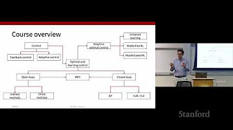
These notes cover Lecture 7 on dynamic programming from Stanford's AA203 course. The instructor took time to set the stage before diving into the algorithm itself — starting with a recap of earlier material, then working through why closed-loop control matters compared to open-loop. Most of the conceptual groundwork happens before any real math appears, and a few distinctions were subtle enough that I had to pause and re-think what was being said. The term dynamic programming shows up throughout as the lecture moves from open-loop methods toward closed-loop policies and the principle of optimality.
 

Recap: open-loop optimal control

 

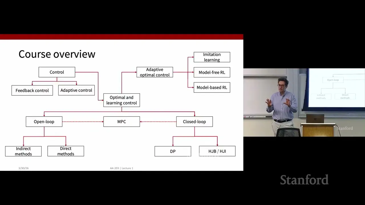
The lecture opened with a review of prior material. Up to this point, the course had focused on one branch of the subject: solving optimal control problems with open-loop approaches. Open-loop means computing a time-indexed sequence of control inputs, chosen to minimize an additive cost function.
 

Two major families of open-loop techniques were covered earlier: indirect methods and direct methods. They complement each other.
 

Indirect methods work by first deriving necessary conditions for optimality. The instructor framed this as extending the familiar nonlinear optimization idea — setting the gradient to zero — into infinite-dimensional optimal control space. Following these conditions leads to a two-point boundary-value problem: a differential equation with boundary conditions split across two different points in time. Indirect approaches date back to the 1960s and 1970s, but they still have value. One big advantage is that they can deliver closed-form analytical solutions. An explicit closed-form optimal control sequence is easy to implement because it requires essentially no runtime computation. The instructor also noted that indirect optimal control ideas can be mixed with other control techniques to create hybrid methods.
 

Direct methods take a different path. You discretize the continuous-time optimal control problem. Once discretized, it becomes a standard nonlinear optimization problem, and you can throw whatever nonlinear numerical solver you prefer at it.
 

For robotics work today, direct methods are far more popular. This comes from advances in both optimization algorithms and computing hardware. Running nonlinear solvers on embedded edge hardware is now realistic — something that wouldn't have been practical decades ago when indirect methods first appeared. Even so, indirect methods retain niche usefulness, especially when closed-form expressions are attainable.
 

With that recap done, the lecturer didn't linger on comparing the two approaches. Instead, the class moved to the other major branch on the conceptual map: closed-loop optimal control.
 

Closed-loop control: policies instead of sequences

 

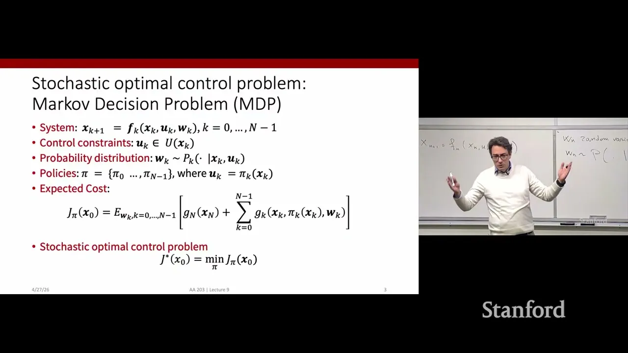
This is where the big conceptual shift happens. The underlying optimal control problem statement doesn't change. What changes is the mathematical object we're trying to compute.
 

In open-loop work, we hunt for a control sequence — a function purely of time. In closed-loop optimal control, the target is an optimal closed-loop policy. A policy is a control law. Given any possible system state you could occupy at time t, the policy tells you what the optimal control action u∗u∗ should be. It maps (time, state) pairs directly to control actions.
 

The instructor flagged that open-loop versus closed-loop can be confusing. There's an important observation here: if the system perfectly follows the nominal trajectory produced by an open-loop control sequence, then executing the corresponding closed-loop policy yields exactly identical behavior. Under perfect nominal conditions, they behave the same.
 

So why go through the extra trouble to compute a closed-loop policy at all?
 

The answer is real-world imperfections. The basic mathematical setup ignores disturbances and model mismatch. But real hardware never perfectly matches simulation models. Noise, external pushes, parameter drift — they all push the system away from the planned trajectory.
 

A closed-loop policy is more robust. If you drift off the nominal path, the policy still knows the best action to take for whatever new state you land in. An open-loop sequence doesn't do that. It blindly applies whatever control was pre-computed for timestamp t, regardless of where the system actually is. If you deviate from the plan, there are no built-in corrections.
 

I found this contrast clear, though I can see how someone might mix it up on first pass. The lecturer even paused to check whether the room was following. An open-loop control value utut​ works great when you sit exactly on the nominal state trajectory. Once you drift away from it, there are no guarantees it's still a good choice.
 

So closed-loop policies offer better robustness against real-world drift. But they come with a steep trade-off: solving for them demands far more computation. That tension set up the rest of the lecture.
 

We want the robustness of closed-loop thinking, but we'd like to avoid the extreme compute cost. The instructor briefly foreshadowed model predictive control (MPC) as an approach that tries to get the best of both — reason with closed-loop ideas while keeping the computational burden closer to open-loop techniques. MPC would be covered a few weeks later.
 

The immediate task for Lecture 7: learn an algorithm for computing optimal closed-loop policies — dynamic programming.
 

Discrete-time setup and the principle of optimality

 

Before deriving dynamic programming, the lecturer switched the formulation to discrete time. Next week's lecture would extend everything back to continuous time.
 

In discrete-time optimal control, time is no longer continuous. We work with stages indexed by k. Stage k corresponds to time tktk​. "Time instant" and "stage" mean the same thing here. You can get discrete-time dynamics by discretizing continuous-time ordinary differential equations. Euler discretization was given as one straightforward method: starting from x˙=f(x,u,t)x˙=f(x,u,t), approximate the time derivative to write a discrete update rule for states.
 

Controls also become discrete. You apply actions only at each stage k. Each control input must sit inside an allowed control set U, which may depend on the current system state. Physical examples included maximum acceleration limits or maximum thrust constraints.
 

The cost function structure stays analogous to the continuous-time case — still additive. You accumulate stage-wise cost at every time step when you occupy state xkxk​ and apply control ukuk​. There's also a terminal cost term that penalizes the final state at the end of the optimization horizon N. This discrete-time cost structure is exactly what you get when you apply direct discretization methods to continuous problems.
 

The key difference is the solution object. Instead of solving for a pre-computed sequence of controls, we want an optimal policy function π∗π∗. It takes your current state and current time stage, and returns the optimal control action for minimizing the additive cost.
 

The lecturer pointed out how deceptively deep this change is. On the surface it sounds like just swapping a sequence for a state-dependent function, but it changes everything about what you compute.
 

So how do we actually compute this policy? The critical insight that enables dynamic programming is the principle of optimality. It's a direct consequence of having an additive cost objective. If the cost structure were different — say, taking the tangent of summed costs — the principle would no longer hold. That balance is interesting: the problem formulation is general enough to model many real-world tasks, yet still carries enough mathematical structure to enable practical algorithms.
 

The principle of optimality sounds almost obvious the first time you hear it, then confusing as you unpack it, then it clicks back into place. In plain language: if you have an optimal multi-step trajectory from starting point A to target E, then any tail sub-trajectory along that optimal path must itself be the optimal solution for the sub-problem starting at the intermediate state.
 

The lecturer walked through a proof by contradiction. Imagine your globally optimal path goes A → B → E. The claim says the segment from B to E must be optimal for the sub-problem starting at B. Suppose for contradiction it's not. Then there exists some better alternative path from B, say B → C → E, with strictly lower cost. If that were true, you could glue A → B onto this better B-to-E path and produce a new A-to-E trajectory with lower total cost. That directly contradicts the premise that A → B → E was already globally optimal. So the supposition must be wrong — the tail has to be optimal for its sub-problem.
 

A student asked a clarifying question here. The principle only applies to tails of the full optimal trajectory. It does not hold for arbitrary sub-segments cut from the middle. Only suffixes running forward toward the final horizon satisfy the property. That's an easy detail to miss when skimming notes.
 

I thought the proof by contradiction was straightforward, but I can see someone glossing over the "only tails" nuance and misapplying the principle later on homework. It's one of those conceptual gotchas the lecture warns about.
 

A noted limitation

 

The lecturer explicitly flagged one hard requirement for everything covered so far: the principle of optimality relies entirely on the cost being additive.
 

If the cost objective is not additive, the whole reasoning falls apart. The instructor gave a quick hypothetical — replace summation with some other nonlinear transformation of cumulative cost, and you lose the property that makes dynamic programming work.
 

This is an important point left hanging in the lecture. The class doesn't explore what to do when costs are non-additive. It simply states the assumption and moves on. In practice, that means dynamic programming as presented here can't be directly deployed for problems with alternative cost structures. There's no workaround, approximation scheme, or modified principle for non-additive objectives in this segment.
 

It's also worth noting that while the principle of optimality gives the theoretical foundation for dynamic programming, the actual backward recursion algorithm steps haven't appeared yet in the transcript. The setup and proof are complete, but the algorithm execution would presumably follow later in the same lecture.

Content Disclaimer: This article is for general reference only and does not constitute professional R&D guidance, production process advice or quality certification. All material performance data has specific test premises; readers should verify parameters against actual equipment and working conditions.