Stanford AA203 Optimal and Learning‑Based Control ｜ Spring 2026 ｜ Lecture 5： Computational Methods — Annotated Lecture Notes & Key Takeaways

Course Information

Institution: Stanford

Original Course: Stanford AA203 Optimal and Learning‑Based Control ｜ Spring 2026 ｜ Lecture 5： Computational Methods

Instructor Bio: Delivered by Prof. Marco Pavone and Dr. Daniele Gammelli, who focus on numerical implementation and real-world deployment of optimal control algorithms.

Course Description: This session explains the computational realization of optimal control. It covers numerical application of Pontryagin’s principle, continuous-time LQR derivation, and walks through the full workflow of solving control problems with coding tools.

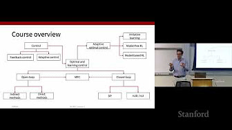
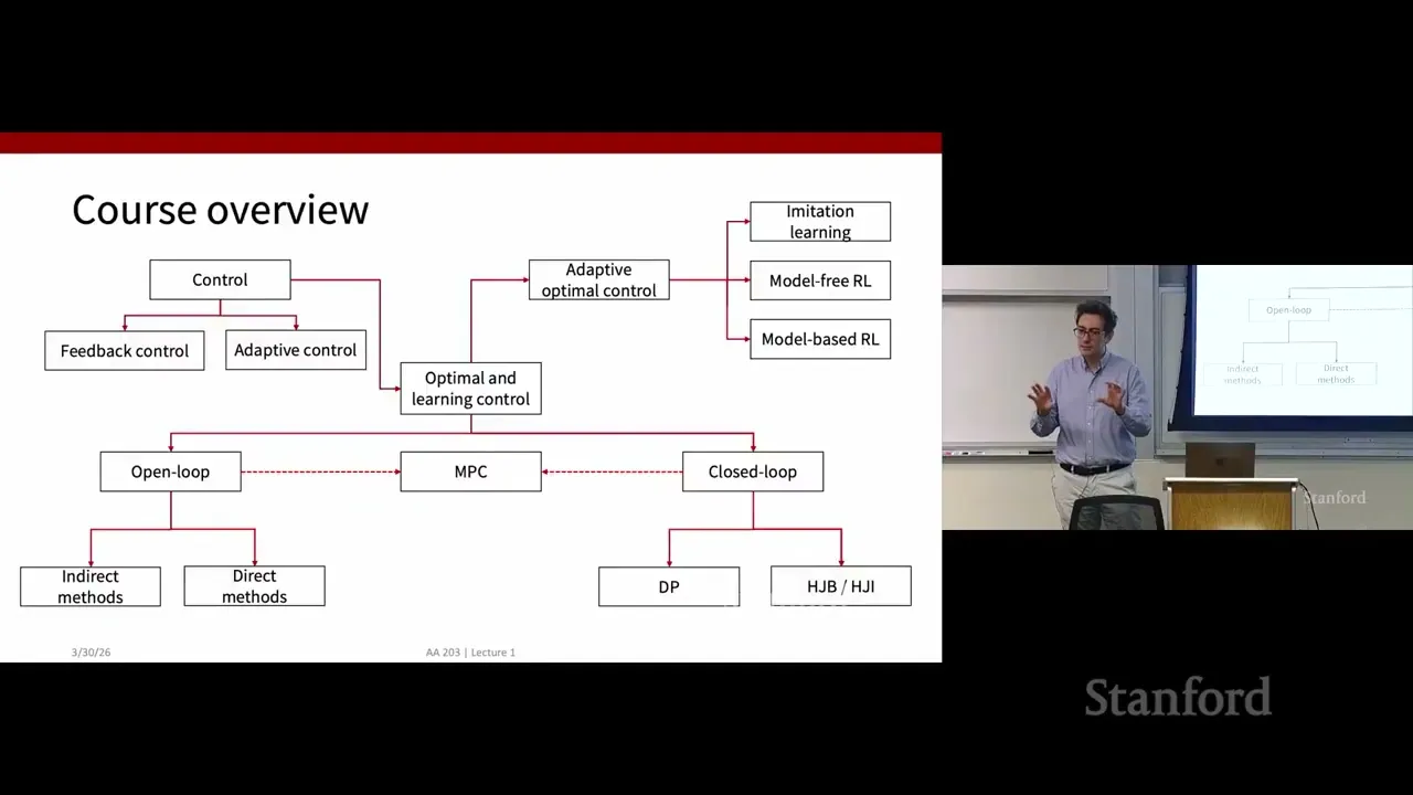
This set of notes covers Lecture 5 for Stanford’s AA203 course, focused on computational methods for optimal control. The lecture picks up in the open‑loop section of the course roadmap, building on indirect methods before shifting toward Pontryagin’s minimum principle. I will walk through the flow of ideas, student‑lecturer exchange, confusing spots, and conceptual comparisons that anchor this computational methods‑focused session.
 

Where We Left Off: Open‑Loop Optimal Control and Indirect Methods

 

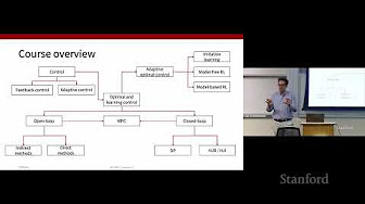
The lecture opens by orienting us to the course schedule. Both the current session and the next day’s class remain within the open‑loop block of the course roadmap. Closed‑loop control will be covered in the following week.
 

The lecturer recaps open‑loop optimal control. An open‑loop optimal control produces a control trajectory u(t) that depends purely on time, not on real‑time system measurements. Our goal is to find this optimal trajectory u(t). The field splits solution approaches into two broad families: indirect methods and direct methods. Last week’s material introduced indirect methods.
 

Indirect methods work in two conceptual steps. First, you derive optimality conditions for the infinite‑dimensional optimal‑control problem. This step draws a parallel to finite‑dimensional optimization. In finite‑dimensional settings, optimality boils down to setting the gradient of your objective function equal to zero. The difference is what these conditions produce. Finite‑dimensional optimization yields algebraic equations. Infinite‑dimensional optimal control gives you differential equations, even though the high‑level intuition stays the same.
 

Indirect methods follow the “optimize‑then‑discretize” workflow. You first derive the optimality conditions, then feed the resulting differential equations into a numerical solver. By contrast, direct methods operate as “discretize‑then‑optimize”. The lecturer notes that today we will wrap our discussion of indirect methods, and then move to direct methods on Wednesday.
 

Before diving into new material, the lecturer revisits the unconstrained optimal‑control problem setup. We aim to find an admissible optimal control u* that drives our system along an admissible state trajectory x. We minimize a cost functional made up of terminal cost H and integrated running‑stage cost G. In the prior lecture, both state and control spaces were assumed to be unbounded.
 

The Hamiltonian is central here, acting like the Lagrangian from finite‑dimensional optimization. It is defined as stage cost plus system dynamics f multiplied by costate functions p(t). These costates are analogous to Lagrange multipliers. One costate variable exists for every state variable in our system.
 

The optimality conditions break into three groups of equations. 1. State dynamics: take partial derivative of Hamiltonian with respect to costate p and recover \(\dot{x}=f\). 2. Costate dynamics: \(\dot{p}\) equals negative partial derivative of Hamiltonian with respect to state x. 3. Algebraic stationarity condition: partial derivative of Hamiltonian with respect to control u equals zero.
 

In practice, people use the third condition to write control u as a function of x and p. Substitute this expression back into the differential equations for x and p, then solve the resulting system. Solving these differential equations requires fixing integration constants, which we do with boundary conditions.
 

Initial‑time boundary conditions are typically given; we know the starting state and starting time. Final‑time boundary conditions change depending on whether final time and final state are fixed or free. If the final state is fixed, there are no admissible perturbations for the final state, which eliminates one set of terms in our boundary‑condition equations.
 

A short student question‑and‑answer interlude happens here. A student references an example from the prior lecture, asking whether the computed final time \(t_f\) corresponded to a genuine optimal control solution, or if the unconstrained nature of the problem meant final time could take arbitrary values. The lecturer clarifies that they had fully solved that example. Once you solve the differential equations, you obtain full solutions for x and p. Since control is a function of x and p, substituting gives you the complete control profile. The lecturer adds an important practical caveat. In that earlier example, the computed optimal control might violate real‑world control magnitude limits, because no control bounds were enforced in that problem formulation. This sets up the main topic for today: bounded‑control constraints.
 

Moving to Bounded Controls and Intuition from Finite‑Dimensional Optimization

 

Up to this point in the course, states and controls had no hard boundaries. The lecturer points out this rarely matches real‑world engineering problems. Actuators have physical limits; you cannot generate infinite thrust. State constraints also show up often, for instance obstacle‑avoidance requirements.
 

Even though state constraints are practically relevant, this lecture will only cover bounds on control inputs. State constraints get skipped for two reasons. First, the mathematical mechanics become far more complicated. Second, indirect methods are not the preferred practical tool for handling state constraints. Engineers will often re‑cast such problems as motion‑planning tasks, where dynamics get simplified or abstracted away. They solve a trajectory‑optimization problem geometrically, and then feed those insights back into indirect‑method solvers.
 

The lecturer builds intuition for bounded controls by drawing analogies back to finite‑dimensional optimization (11:20). For an unconstrained local minimum candidate, any small displacement \(\Delta x\) is allowed, both positive and negative directions. We approximate objective‑function change with a first‑order Taylor expansion: function value change ≈ gradient transposed times displacement, plus higher‑order terms. For a local minimum, any feasible small displacement must increase the objective function value. When you can move freely in both directions, the only way this holds is for the gradient to be zero.
 

This logic breaks when constraints create boundaries. If your optimum sits exactly on the boundary of your feasible set, you cannot take displacements in every direction. You may only perturb your variable in one admissible direction. In this scenario, the gradient no longer has to equal zero. The weaker requirement is that the first‑order change (differential) must be greater than or equal to zero for every feasible displacement. The lecturer uses a visual thought‑experiment example: a function defined over a bounded interval. Points sitting right at the interval edges can qualify as local minima even with non‑zero gradient, because only outward perturbations are forbidden. Only inward moves are allowed, and those inward moves increase the cost value.
 

This finite‑dimensional reasoning translates directly to calculus of variations for infinite‑dimensional optimal‑control problems. In variational optimal‑control, we look at variations \(\delta J\) of our cost functional J. A candidate solution is a relative minimum when the first‑order cost increment is non‑negative. In the earlier unconstrained setup, we could take arbitrary variations \(\delta u\), so we required \(\delta J=0\).
 

Now we face bounded controls. Our control itself is a function of time, so variations \(\delta u(t)\) are also functions. If our control sits strictly inside the allowed bounds at a given time point, we can perturb u both upward and downward, exactly like unconstrained optimization. But if the control lands right on a constraint boundary, only one direction of variation stays admissible. You cannot push the control further past its hard limit. That means one‑sided variations apply for portions of the control profile that touch saturation bounds. This changes our optimality conditions, and this modified set of conditions leads us toward Pontryagin’s minimum principle.
 

Conceptual Gap and Unanswered Points in This Lecture Segment

 

I noticed one point that felt under‑explained in the lecture. The lecturer clearly establishes that boundary‑saturated controls lead to one‑sided admissible variations. But they stop short of showing exactly how that one‑sided variation condition mathematically transforms the old stationarity condition \(\partial H/\partial u = 0\) into Pontryagin’s minimum principle. The lecture builds the analogy very thoroughly, yet does not complete the derivation within the transcribed segment.
 

This is not a mistake in the lecture; the lecturer signals that concrete examples are coming in subsequent slides. Still, for someone watching this lecture without access to those following slides, there is a conceptual leap. You understand why the old condition fails, but you have not yet seen the exact mathematical replacement.
 

Another small open item comes from the state‑constraint discussion. The lecturer says indirect methods are not the tool of choice for state constraints, and people often switch to motion planning. But they do not elaborate on how you practically combine motion‑planning outputs with indirect optimal‑control solvers. This is a high‑level conceptual hint without procedural detail. If you wanted to implement that workflow, you would need to seek extra reading or later course material.
 

The student Q&A also hints at a practical gotcha. Solving an unconstrained optimal‑control problem can produce mathematically valid solutions that are physically unrealizable because control magnitude exceeds actuator limits. You cannot just blindly take indirect‑method answers and deploy them on hardware. You have to check whether your solution respects actuator bounds, and if not, you need to incorporate those bounds into your problem formulation.
 

Variations of Control Functions Under Input Bounds

 

The lecturer spends time unpacking what a variation \(\delta u(t)\) means when u(t) is subject to hard upper bound \(\bar u\).
 

Your control trajectory u(t) can have three different types of time segments. 1. Control sits strictly inside bounds: both positive and negative variations \(\delta u\) are allowed. 2. Control sits exactly on the upper boundary: you may only apply negative variations; pushing further positive violates constraints. 3. Control sits exactly on a lower boundary: only positive variations remain admissible.
 

Different time segments of the same control trajectory can fall into different categories. Parts of the trajectory run inside feasible set, other parts stick to constraint boundaries. These boundary‑touching intervals are known as “bang‑bang” segments in optimal‑control terminology, though the lecturer does not use that exact word in this transcript.
 

This means the optimality condition is no longer uniform across the whole time horizon. At times where control lies interior to constraints, we still recover the stationarity condition we learned for unbounded controls. At times when control hits the boundary, we only enforce the one‑sided inequality condition on variations of J.
 

This conceptual groundwork sets up Pontryagin’s minimum principle. The minimum principle gives the correct optimality condition for problems with hard control bounds. Instead of requiring derivative of Hamiltonian with respect to u equal zero everywhere, we require that the Hamiltonian is minimized over the feasible set of control inputs at every instant of time.
 

The transcript cuts off before showing the full mathematical statement and worked examples, but all the conceptual building blocks are laid out. The finite‑dimensional constrained‑optimization analogy is the main mental model you carry forward.
 

The lecture also reminds us of the big‑picture computational‑methods theme tied to indirect methods. Indirect methods require you to derive all optimality conditions by hand first. You then assemble a boundary‑value differential‑equation problem and hand it to numerical solvers. That whole “optimize‑then‑discretize” pipeline contrasts sharply with direct methods which discretize the problem first and then run numerical optimization on a finite‑dimensional decision vector. Direct methods will be covered in the upcoming Wednesday lecture.
 

For indirect methods, the heavy‑lifting human work happens at the derivation phase. If your problem changes (adding control bounds, different cost functions), you have to re‑derive optimality conditions before you can use numerical solvers. That is one practical weakness of indirect approaches, which direct methods partly alleviate.

Content Disclaimer: This article is for general reference only and does not constitute professional R&D guidance, production process advice or quality certification. All material performance data has specific test premises; readers should verify parameters against actual equipment and working conditions.