AStanford AA203 Optimal and Learning‑Based Control ｜ Spring 2026 ｜ Lecture 8： LQR‑Style Algorithms — Annotated Lecture Notes & Key Takeaways

Course Information

Institution: AStanford

Original Course: AStanford AA203 Optimal and Learning‑Based Control ｜ Spring 2026 ｜ Lecture 8： LQR‑Style Algorithms

Instructor Bio: Taught by Prof. Marco Pavone and Dr. Daniele Gammelli, who conduct in-depth research on LQR-family algorithms for robotic control applications.

Course Description: This lecture covers extended LQR algorithms, including iterative LQR (iLQR) and Differential Dynamic Programming (DDP) for nonlinear systems. It derives LQR variants for tracking tasks and demonstrates use in robotic trajectory optimization.

These notes cover Stanford AA203 Lecture 8 focused on LQR‑Style Algorithms. I’ve broken down what the instructor walked through, flagged confusing spots, and captured the student Q&A exchanges from the lecture recording. This lecture does not dive into brand‑new optimal‑control theory from scratch. Instead, it expands on LQR, showing how to reuse this tool across many practical control problems.
 

Lecture roadmap and course forward planning

 

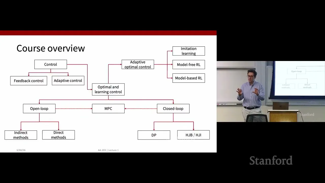
The instructor opened by recalling material from the prior Monday lecture. Back then, the class viewed optimal control problems from a closed‑loop perspective, where we optimize for a closed‑loop control policy. That session introduced dynamic programming as the core tool for solving for closed‑loop optimal policies, built for discrete‑time problem formulations.
 

Plans for future lectures got laid out early on. In the coming week, the class will extend dynamic programming ideas into continuous‑time mathematics, landing at the Hamilton‑Jacobi‑Bellman equation plus reachability theory. Further down the schedule, they will cover stochastic formulations where system dynamics get disturbed by random noise. That segment will teach the stochastic version of dynamic programming equations, which many students might have seen in prior coursework focused on decision‑making under uncertainty. The Wednesday lecture of the following week will handle continuous‑time closed‑loop optimal control, expanding dynamic programming into the continuous‑time HJB framework, and after that the course will move into MPC content.
 

Assignment work ties directly to these concepts. Problem Set 2 gives students hands‑on practice with both dynamic programming and LQR. One exercise quantifies the computational savings dynamic programming delivers compared to brute‑force solution search. Another task requires students to write an LQR implementation completely from scratch. The instructor acknowledged that AI tools could generate this code, but emphasized the educational value of building it manually at least one time.
 

Today’s lecture would not introduce brand‑new optimal‑control fundamentals. Every minute would centre on practical ways to deploy LQR across diverse control scenarios. LQR is not merely a textbook thought experiment; it sees heavy real‑world use across controls, robotics and adjacent technical fields.
 

LQR basics and generalised cost‑function forms

 

Standard LQR is built for regulator tasks. Its native objective pushes system states toward the origin, hence the full name linear‑quadratic regulator. This works great for some simulation examples. But real‑world robotic systems rarely care about forcing every state variable to zero. More often we want to track a predefined desired behaviour or a reference trajectory. The instructor confirms LQR can be adapted for trajectory‑tracking jobs, and a big chunk of this lecture unpacks exactly how that adaptation works.
 

A student raised a quick question comparing LQR against simple proportional‑only (P) controllers. They asked why practitioners would pick LQR over P‑control. The instructor pointed out a core difference. Basic P‑controllers lack an explicit objective function. You can indirectly tweak system response through gain tuning. Students in foundational engineering courses spend lots of time mapping phase margin, gain margin, pole placement to time‑domain behaviours like rise‑time. But this whole workflow remains indirect.
 

LQR hands you clear, explicit knobs to define your optimisation objectives. Beyond stabilisation jobs, it handles trajectory tracking, and you can even repurpose it to compute whole optimal trajectories. The instructor stressed these two families of controllers are not rivals. They operate at different layers within a typical control hierarchy.
 

P‑control frequently sits at the lowest layer, directly commanding actuators like throttles or steering mechanisms. LQR and similar trajectory‑optimisation tools sit one layer higher. They deal with trajectory generation. Even higher layers handle high‑level decision‑making. These top‑level decision layers might use decision‑making theory, or modern data‑driven approaches such as large language and vision‑language models. Each layer operates at a different granularity when reasoning over the physical dynamics of the hardware. The instructor used a human‑movement analogy: when your brain decides to walk toward a door, you don’t consciously compute every single arm joint displacement. That fine‑grained dynamic computation happens at lower control layers.
 

Moving into the formal LQR recap. LQR addresses a specific class of optimal‑control problem. It assumes no hard constraints on states or control inputs. System dynamics are linear, written as \(x_{k+1}=A_kx_k+B_ku_k\). Important detail: matrices \(A_k\) and \(B_k\) can change with time; this is time‑varying dynamics, not limited to time‑invariant systems. That property becomes important for later extensions.
 

The baseline cost function includes a quadratic terminal‑state penalty plus running cost terms with quadratic penalties on state and on control effort. The instructor then walked through generalising this cost function. You can insert cross terms mixing state and control variables (x times u). These cross terms do not break the overall derivation flow. One practical motivation: sometimes how heavily you penalise control effort depends on what state the system currently occupies. More critical for our use‑case: these cross terms naturally pop up whenever we perform linearisation steps for trajectory‑tracking work.
 

With cross‑term cost, the Bellman equation still applies. We start from our known quadratic terminal‑cost boundary condition. We take gradients, set gradients equal to zero, solve for control input, substitute that solution back into Bellman’s equation. The cost‑to‑go remains quadratic. The optimal control law stays linear state feedback. Only the numerical values for gain matrices L and Riccati‑solution matrix P shift. The exact updated matrix formulas are messy algebra‑wise, so the instructor said they would not write them all on slides. Full equations live in the lecture notes referenced on the slide deck and in the course syllabus.
 

The generalisation does not stop at cross terms. We can add linear terms in state, linear terms in control, plus constant offset terms to our cost expression. We can also shift our dynamics to affine form: \(x_{k+1}=A_kx_k+B_ku_k+d_k\). The extra term \(d_k\) acts like a known disturbance signal; imagine a predicted wind gust hitting your robot at timestep k.
 

We repeat the exact same Bellman‑equation derivation workflow for this affine‑dynamics setup. Our boundary condition now combines quadratic, linear, and constant components. After solving and substituting back, our optimal control policy changes form. It keeps the familiar linear feedback piece, but now gains an extra feed‑forward offset term. The optimal cost‑to‑go is no longer purely quadratic; it includes linear terms in state plus a constant offset value.
 

There was some back‑and‑forth student discussion about notation during this segment. Different matrix symbols appear in the generalised cost compared to the prior lecture. The instructor clarified this is mostly a notation detail. All these weighting matrices (Q, R, H, \(Q_N\)) are design parameters the control engineer selects.
 

This brings up the topic known as LQR tuning. Once you set all your cost‑function weight matrices correctly, the math automatically outputs your optimal control policy and associated optimal cost. The real challenge is picking those weight matrices in the first place. That choice is not always obvious. The instructor shared a real‑world anecdote: tuning an LQR‑based tracking algorithm for a vehicle‑style platform took multiple calendar months. Engineers iterated to get satisfying lateral and longitudinal handling behaviour. The system needed to keep safety guarantees, but also deliver smooth, pleasant handling for human end‑users. Tuning mixes heuristic judgment and simulation‑based testing. All those matrices are just symbolic placeholders that the designer must set appropriately.
 

Even more generalised cost forms bring additional design vectors: constant offset vectors and coefficient matrices that can come from designer choice, or alternatively emerge automatically from linearisation when we solve tracking problems. The derivation logic stays identical. If you work through the math yourself, you find that control law still contains linear state feedback plus that feed‑forward term. There exists an intuitive physical reading for this combined feedback‑plus‑feedforward structure, which the instructor promised to unpack later in lecture. The cost‑to‑go expression likewise expands, retaining its quadratic core but appending linear terms and scalar constants. All these new matrix and vector quantities get solved via modified Riccati‑style update recursions. The detailed update math lives again in the written lecture notes because the algebraic expressions become cumbersome to present verbally.
 

Key takeaways and unresolved points from the lecture

 

The high‑level takeaway from this whole generalisation block is straightforward. LQR can accept richer cost structures (cross terms, linear terms, constants) and can work with affine dynamics. The overall structure of the optimal solution barely changes. The main additions are feed‑forward terms in control law and linear plus constant pieces inside the cost‑to‑go function. All heavy‑lifting update equations are delegated to the course’s written lecture notes.
 

One point I found a bit hard to follow is exactly when you would manually choose those extra cross‑terms, linear‑cost terms versus when they just show up as a by‑product of linearisation for tracking. The instructor mentions both scenarios, but concrete small worked examples would have helped solidify the distinction. Right now the reasoning is conceptual, without numbers to illustrate.
 

There is also an open practical question touched on but not resolved within this lecture segment. Tuning LQR weight matrices is acknowledged to be difficult and time‑consuming. The instructor mentions simulation as one tool, but does not go over any structured tuning workflows or heuristics. This leaves hanging how new engineers should approach this tuning task in practice. We know it takes effort, but the lecture does not give actionable step‑by‑step guidance.
 

Looking ahead in the course material. After finishing this generalised LQR foundation, the lecture will move to iterative LQR (iLQR), a widely‑used algorithm, and then its further refinement known as differential dynamic programming (DDP). Both iLQR and DDP build entirely upon core LQR insights.

Content Disclaimer: This article is for general reference only and does not constitute professional R&D guidance, production process advice or quality certification. All material performance data has specific test premises; readers should verify parameters against actual equipment and working conditions.