Stanford AA203 Optimal and Learning-Based Control | Spring 2026 | Lecture 17: RL Value-Based Methods — Annotated Lecture Notes & Key Takeaways

Course Information

Institution: Stanford

Original Course: Stanford AA203 Optimal and Learning-Based Control | Spring 2026 | Lecture 17: RL Value-Based Methods

Instructor Bio: Delivered by Prof. Marco Pavone and Dr. Daniele Gammelli, with rich research outcomes on value-based reinforcement learning algorithms.

Course Description: This session focuses on value-based RL methods, covering the principles and improvements of Q-learning and DQN. It analyzes bias and variance in value function estimation, and covers engineering best practices for deep value-based algorithms.

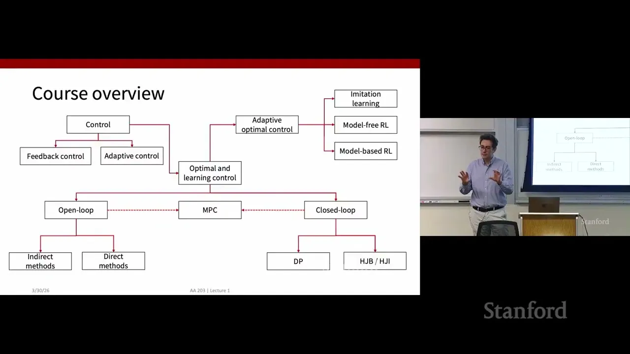
This is Lecture 17 of Stanford’s AA203 Optimal and Learning-Based Control, and it marks a deep dive into value-based methods for reinforcement learning (RL). After spending earlier weeks on imitation learning and the basic foundations of RL, the lecturer uses this session to move from pure prediction (estimating value functions) to actual control (finding optimal policies) with model-free algorithms. The lecture builds slowly, starting with a recap of last week’s core ideas before landing on SARSA — one of the most classic value-based RL algorithms — and teeing up Q-learning, the on-policy/off-policy distinction, value function approximation, and a quick look at deep RL.
 

Recap: Building Blocks of Value-Based RL Methods

 

The lecture opens by retracing the road map of the past few weeks. The class started with imitation learning, where the goal is to mimic an expert’s behavior. Then it moved into reinforcement learning: learning through trial and error, without a pre-built model of how the environment works.
 

Two core goals have run through all the recent material: prediction and control. Prediction means taking a fixed policy and estimating how much total reward you can expect from each state. Control is the real end goal: searching for the policy that maximizes performance.
 

The lecturer reminds everyone that dynamic programming gives exact solutions to these problems — policy iteration and value iteration, built on the Bellman optimality principle. These work perfectly, but they have one giant limitation: you need perfect knowledge of the system’s transition dynamics. You have to know exactly how likely each next state is, given any current state and action. For most real control problems, that information isn’t available.
 

That’s why model-free RL exists. You learn directly from interacting with the environment, no dynamics model required. Last week introduced two foundational approaches to this: Monte Carlo learning and temporal difference (TD) learning.
 

Monte Carlo learning is conceptually simple. You run an entire episode until you hit a terminal state, add up all the discounted rewards along the way, and use that total return as the target to update your value estimate. It’s an unbiased estimate, but it has high variance. Every random step along the episode adds noise to the final total. You also can’t learn anything until the whole episode is over.
 

TD learning takes a different approach, borrowing the bootstrap idea from dynamic programming. Instead of waiting for the end of the episode, you update your value guess using just the immediate reward plus your current estimate of the next state’s value. It’s a one-step lookahead.
 

The lecturer highlights two key advantages of TD learning. First, it has lower variance than Monte Carlo, because you’re only sampling one step of randomness instead of a whole episode’s worth. Second, you can update online, step by step, even with incomplete sequences. You don’t need to reach a terminal state to make progress on learning.
 

Everything said about state value functions applies equally to action-value (Q) functions, which map state-action pairs to expected total reward. Q-functions are what make control algorithms work, because they let you pick the best action in any given state.
 

All of this feeds into the general framework for control: generalized policy iteration. You alternate between two steps. First, policy evaluation: estimate the value function for your current policy. Second, policy improvement: update the policy to act greedily with respect to that value function, usually with some epsilon-greedy exploration to make sure you don’t miss better options. Repeat this cycle enough times, and you converge toward the optimal policy and optimal value function.
 

Monte Carlo control is the simplest version of this framework: use Monte Carlo for evaluation, epsilon-greedy for improvement.
 

The lecturer also name-checks the standard references for the field: Sutton and Barto’s textbook on reinforcement learning, and David Silver’s popular course, noting that some of the day’s slides draw inspiration from Silver’s material.
 

SARSA: Turning TD Learning Into a Control Algorithm

 

If TD learning works better than Monte Carlo for prediction, the natural question is: why not use it for control too? That’s exactly the step that leads to SARSA, one of the most well-known algorithms in reinforcement learning.
 

The name comes from the five pieces of data you need for every update: state, action, reward, next state, next action. Run those five letters together and you get “SARSA.”
 

The algorithm itself is a straightforward twist on Monte Carlo control. You still follow the generalized policy iteration pattern. The only real change is replacing the Monte Carlo evaluation step with one-step TD updates, applied at every time step instead of at the end of an episode.
 

The lecturer walks through the logic of the pseudocode. You start by initializing your Q-function — you can set all values to zero, or any arbitrary starting point. Then you start an episode in some initial state.
 

From that state, you pick an action using your current epsilon-greedy policy. Most of the time you choose the action with the highest Q-value, but with probability epsilon you pick a random action to keep exploring.
 

You take that action, receive a reward, and land in the next state. Then, critically, you pick the next action using that same epsilon-greedy policy. Now you have all five elements you need for the update.
 

The update rule follows the TD pattern. You adjust your estimate of Q(s,a) to move closer to the target: the immediate reward plus gamma times your estimate of Q(s’, a’).
 

Then you shift forward one step. The next state becomes your current state, the next action becomes your current action, and you repeat until the episode ends.
 

To build intuition for how this works in practice, the lecturer walks through a windy grid world example. The setup is standard: an agent moves on a grid in four cardinal directions, trying to reach a goal cell as quickly as possible. Every time step gives a reward of -1, so minimizing travel time is equivalent to maximizing total reward. The discount factor gamma is set to 1.
 

The twist is the wind. A fictitious wind blows upward from the bottom of the grid, and each column has a different wind strength. In some columns the wind does nothing; in others it pushes the agent up one cell, or more, every step.
 

The lecturer pauses to ask the audience what the optimal path would be. Most people’s first instinct is to head straight toward the goal. That intuition turns out to be wrong.
 

If you try to cut across horizontally while low in the grid, the wind keeps pushing you upward every step. You can overshoot, or get pushed past the goal entirely. The actual optimal strategy is counterintuitive at first: you first push all the way up to the top edge of the grid, then work your way back toward the goal from there.
 

I found this example really useful. It drives home why you need learning algorithms at all — even in a tiny, simple environment with transparent rules, the optimal policy isn’t obvious if you just glance at the setup.
 

The lecturer confirms that SARSA does converge to the optimal policy on this problem, under the right conditions.
 

What’s Next: Q-Learning and the On-Policy / Off-Policy Divide

 

SARSA is only half the story of this lecture. The second major algorithm on the agenda is Q-learning, and comparing the two is how the lecturer unpacks one of the most important distinctions in reinforcement learning: on-policy versus off-policy methods.
 

SARSA is an on-policy algorithm. The policy you use to take actions and collect data is the exact same policy you’re evaluating and improving. You learn about the epsilon-greedy policy by following the epsilon-greedy policy.
 

Q-learning is off-policy. You can learn about the optimal greedy policy while still behaving according to an exploratory epsilon-greedy policy. The policy you act with doesn’t have to match the policy you’re learning about.
 

The transcript cuts off right as this comparison gets into detail, but the lecture’s opening roadmap makes clear this is the central conceptual takeaway of the session.
 

The roadmap also teases two more topics that come later in the lecture. First, value function approximation. All the algorithms discussed so far are tabular — they store a separate value for every state and every action. That works for tiny grid worlds, but it breaks completely when state and action spaces are large, continuous, or high-dimensional. Approximating the value function with a parameterized model lets you scale these methods to real-world control problems.
 

Second, the lecture wraps up with a brief look at deep reinforcement learning methods and applications, connecting these classic tabular algorithms to the modern techniques used in robotics, games, and industry.
 

Points Worth Pausing On

 

There are a few spots in this lecture where it’s easy to get stuck, or where the lecturer skips over details that matter if you want to work with these algorithms yourself.
 

First, the windy grid world intuition gap. The lecturer calls out that most people get the optimal path wrong on their first guess, and that’s exactly the point. It’s surprisingly hard to reason through even simple environmental dynamics by hand. If you found yourself skeptical of the “hug the top edge” strategy when it was first described, that’s a normal reaction. It takes walking through a few steps of wind displacement to see why it works.
 

Second, the on-policy versus off-policy distinction. The lecturer frames it as the key difference between SARSA and Q-learning, but this segment of the talk doesn’t fully lay out the practical tradeoffs. It’s easy to memorize which algorithm is which category, but harder to immediately grasp why that difference changes things like sample efficiency, convergence behavior, and safety in risky environments. This is a topic that likely clicks fully once you see Q-learning worked out end to end.
 

Third, convergence conditions. The lecturer states that SARSA converges to the optimal policy, but doesn’t list the assumptions required for that guarantee. In practice, tabular SARSA only converges reliably if you decay the learning rate appropriately over time, gradually reduce epsilon to shift from exploration to exploitation, and visit every state-action pair enough times. Use a fixed learning rate and fixed epsilon, and you might just oscillate forever. The Sutton & Barto textbook and David Silver’s course both cover these conditions in depth.
 

All in all, this lecture grounds you in the core mechanics of value-based methods for reinforcement learning, starting with the foundations of TD learning and building up to the SARSA control algorithm. It sets up the most important contrast in model-free RL — on-policy versus off-policy learning — and points toward the approximation techniques that make these methods work for real, high-dimensional control problems. If you follow along with the Q-learning discussion and the function approximation material that comes next, you’ll have a complete picture of the standard value-based RL toolkit.