Stanford AA203 Optimal and Learning-Based Control ｜ Spring 2026 ｜ Lecture 18： RL Policy Optimization — Annotated Lecture Notes & Key Takeaways

Course Information

Institution: Stanford

Original Course: Stanford AA203 Optimal and Learning-Based Control ｜ Spring 2026 ｜ Lecture 18： RL Policy Optimization

Instructor Bio: Taught by Prof. Marco Pavone and Dr. Daniele Gammelli. Policy optimization is one of their core research directions in reinforcement learning.

Course Description: This lecture provides an in-depth look at RL policy optimization, including the Actor-Critic framework and advantage function design. It discusses policy gradient improvements, and covers architecture design and real-world applications of deep policy algorithms.

This set of notes covers Lecture 18 of Stanford's AA203 Optimal and Learning-Based Control course from Spring 2026. The lecture lands during the final week of the semester and shifts focus from value-based reinforcement learning to the second major branch of model-free RL: policy optimization. The lecturer walks through the full mathematical derivation of policy gradients, builds up to the basic REINFORCE algorithm, and previews more advanced methods that address its limitations.
 

Framing policy optimization as a parametric learning problem

 

Up to this point, all the model-free RL methods in the course have fallen into the value-based family. In those approaches, you never define the policy directly. Instead, you learn a value function or Q-function, and the optimal action at any state is whichever one gives the highest estimated value. The policy exists implicitly, buried inside the value estimates.
 

Policy optimization takes the opposite approach. Here the policy is represented explicitly as a parametric function, written π_θ, where θ is a vector of tunable parameters. The goal is to adjust θ directly to maximize the RL objective.
 

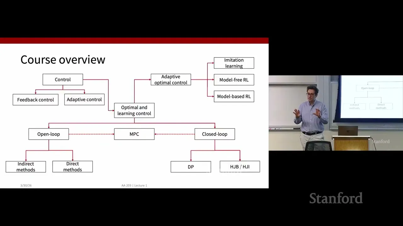
The lecturer positions this as the natural next step in the course roadmap. The past few weeks have worked through learning-based methods for optimal control — starting with Monte Carlo and temporal difference learning, then expanding into full value-based algorithms. Policy optimization completes the model-free RL picture.
 

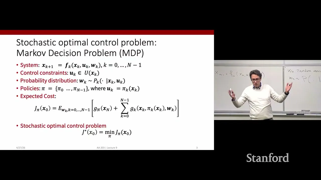
To set the stage, the lecturer recaps the standard MDP formalism. An agent interacts with an environment over time, producing trajectories of states and control actions. Randomness enters from three places: the distribution of initial states (like starting conditions in a Gym simulation), the stochastic policy itself, and the environment's transition dynamics. Together, these three sources define a probability distribution over every possible trajectory the agent could take.
 

The RL objective is to maximize the expected sum of discounted cumulative rewards under this trajectory distribution. In the policy optimization setting, this objective becomes a function J(θ), and the task reduces to finding the parameter vector θ that makes J(θ) as large as possible. For simplicity, the derivation uses an undiscounted reward setup, but the lecturer notes that all results carry over straightforwardly when discounting is included.
 

The core math behind policy gradients

 

If we want to maximize J(θ) with gradient ascent, the first thing we need is an expression for the gradient of J with respect to θ. Most of the lecture is spent deriving this into a form we can actually compute.
 

At first glance, the gradient looks impossible to calculate directly. It's an integral over all possible trajectories, weighted by their probability, and we don't know the environment's transition dynamics. The lecturer introduces a standard identity to reframe the problem: the gradient of a probability density can be rewritten as the density itself times the gradient of its logarithm.
 

Substituting this identity into the gradient of J(θ) rearranges the integral into an expectation. Instead of integrating the gradient of trajectory probability times reward, we take the expectation of the gradient of log trajectory probability times reward, under the trajectory distribution. A small algebraic shift, but it's the key that makes the whole approach work.
 

We still need to unpack the gradient of log P(τ). Using the factored form of trajectory probability, the logarithm turns the product of terms into a sum. Log P(τ) breaks cleanly into three separate sums: one for the initial state probability, one for the policy at each time step, and one for the transition dynamics at each step.
 

This is where the big simplification happens. Only the policy terms depend on θ. The initial state distribution and the environment transition dynamics are properties of the world, not of our policy. Their gradients with respect to θ are exactly zero, so they drop out entirely.
 

After removing those terms, we're left with a policy gradient equal to the expected value of the sum of ∇ log π(a_t | s_t) across time, multiplied by the total reward of the full trajectory. Every piece inside this expectation is something we can compute ourselves, as long as we know the form of our parametric policy. For example, with a Gaussian policy for continuous control, θ represents the mean and standard deviation of the action distribution, and we can write exact formulas for both log π and its gradient.
 

I found this section moves fastest right when the terms start canceling. If you're not following the algebra line by line, it's easy to miss why the transition dynamics vanish from the gradient. The short version: changing your policy doesn't change how the environment responds to an action, so those terms don't affect how the objective changes with θ.
 

The REINFORCE algorithm

 

We now have a clean expression for the policy gradient, but it's still an expectation over the trajectory distribution. Since we can't compute that expectation analytically, we use the same sampling trick used everywhere else in RL: approximate it with an empirical average.
 

Run the current policy N separate times in the environment, and you get N sample trajectories. For each trajectory, calculate the sum of ∇ log π terms multiplied by that trajectory's total reward. Averaging this across all N rollouts gives an unbiased estimate of the true policy gradient.
 

This is the core idea behind REINFORCE, the first fully worked policy optimization method in the lecture. The algorithm follows a simple repeating cycle:

• Roll out the current policy N times to collect a batch of trajectories.

• Compute the sample-based estimate of the policy gradient from the batch.

• Update θ by taking a step in the direction of the gradient.

Conceptually, REINFORCE works by making actions that led to high-reward trajectories slightly more probable, and actions that led to low-reward trajectories slightly less probable. Over many iterations, the policy drifts toward better expected performance.
 

Limitations and what's next

 

REINFORCE is clean and intuitive, but it has significant weaknesses that limit real-world use. The lecturer highlights variance as the biggest practical problem. Each trajectory is a single noisy sample of the true expected return, so the gradient estimate can bounce around dramatically between batches. High variance slows learning and can cause the policy to collapse entirely if step sizes aren't tuned carefully.
 

This lecture only covers vanilla REINFORCE to illustrate the core policy gradient idea. The next major topic is actor-critic methods, described as extremely popular variants of policy optimization. Actor-critic algorithms learn a value function alongside the policy and use that value function to reduce the variance of the gradient estimate. This fixes the main flaw of basic REINFORCE, at the cost of adding another learned function to the system.
 

The lecture wraps up by noting that after actor-critic, the course will touch on more modern RL algorithms and real-world applications before the semester ends.
 

One point that felt slightly hand-wavy: the lecturer states multiple times that the undiscounted derivation extends easily to discounted rewards, but never shows exactly where the discount factor slots into the final gradient formula. Not a hard step to work out on your own, but a gap in the in-lecture derivation if you're trying to follow every line of math.
 

Overall, this lecture builds the complete foundational theory for RL policy optimization, starting from the basic MDP objective and ending with a functional iterative algorithm. REINFORCE itself is rarely used in its simplest form today, but every modern policy gradient approach builds on the exact same mathematical steps walked through in this session.

Content Disclaimer: This article is for general reference only and does not constitute professional R&D guidance, production process advice or quality certification. All material performance data has specific test premises; readers should verify parameters against actual equipment and working conditions.