Stanford AA203 Optimal and Learning-Based Control ｜ Spring 2026 ｜ Lecture 13： Intro to Learning — Annotated Lecture Notes & Key Takeaways

Course Information

Institution: Stanford

Original Course: Stanford AA203 Optimal and Learning-Based Control ｜ Spring 2026 ｜ Lecture 13： Intro to Learning

Instructor Bio: Delivered by Prof. Marco Pavone and Dr. Daniele Gammelli, who specialize in data-driven control methods and related curriculum design.

Course Description: This session introduces foundational concepts of learning-based control. It covers system identification and basic regression models, explains how to learn system dynamics from data, and paves the way for learning-based control methodologies.

Lecture 13 marks the official start of the second module in Stanford's AA203 course, moving away from the classic optimal control methods that dominated the first half and into learning-based control. For the first seven weeks, every approach we discussed assumed a perfect, analytical description of the system dynamics. This lecture explains why that assumption doesn't always hold, lays out three broad strategies for handling uncertainty, and maps the landscape of learning-based methods for the rest of the semester.
 

Three ways to handle uncertainty

 

To set up the problem, the lecturer first recapped the methods already covered and where they fall short.
 

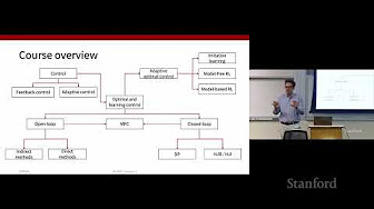
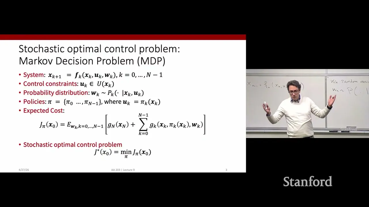
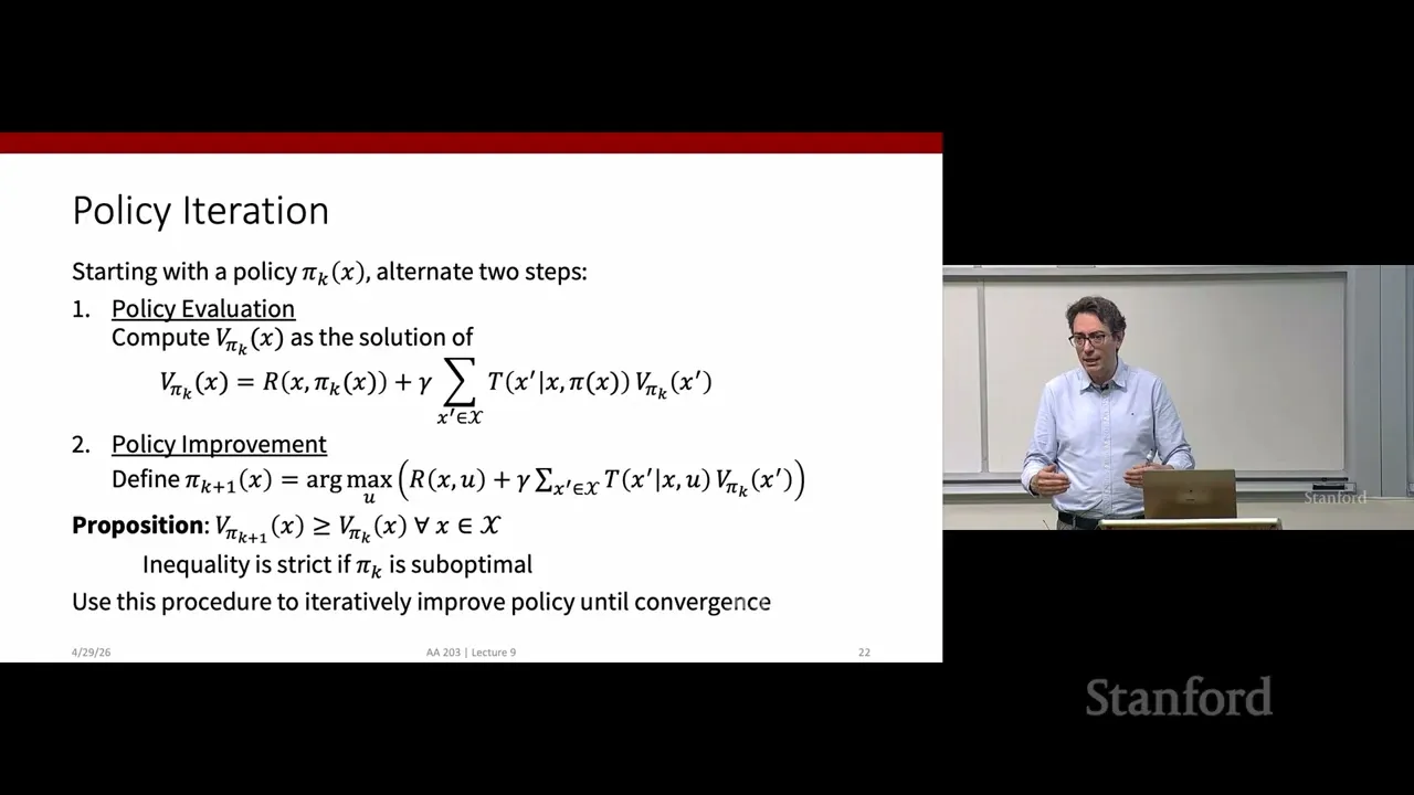
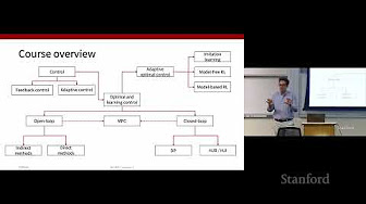
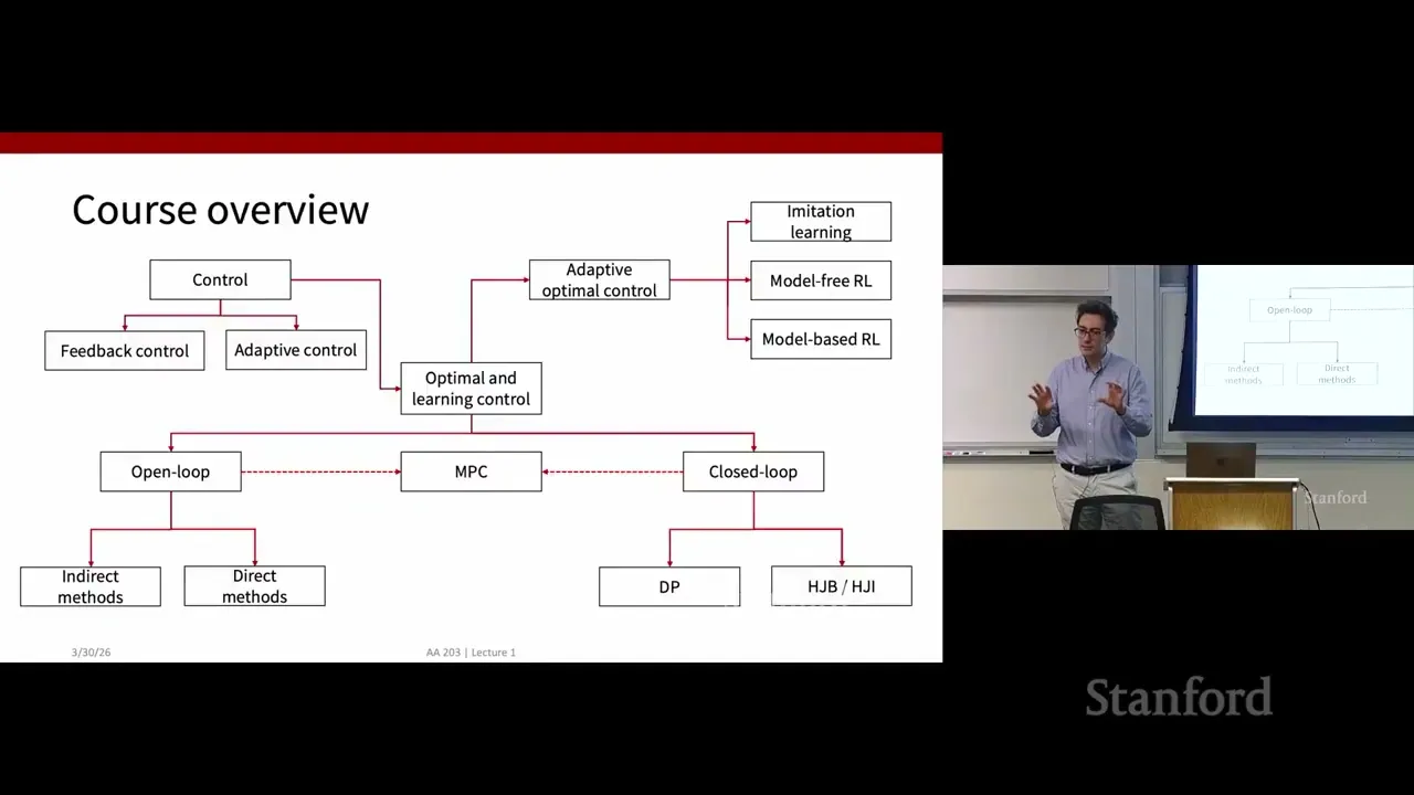
Open-loop methods compute a single optimal trajectory from a given starting state. They're fast and reliable, but only work for that exact initial condition — change the starting point even a little, and the whole trajectory has to be recomputed. Closed-loop methods like dynamic programming and Hamilton-Jacobi-Bellman equations go further, computing a full control policy that maps every possible state to an optimal action. That's much more powerful in principle, but comes with steep computational cost. Model predictive control sits in the middle, getting closed-loop performance by repeatedly solving open-loop problems online at each time step.
 

All of these methods degrade, or even fail entirely, when the system doesn't behave exactly like the mathematical model. Real systems have unmodeled disturbances, unknown physical parameters, and messy real-world effects that can't be cleanly written down as differential equations.
 

The lecturer walked through three high-level approaches to this problem, ordered from simplest to most sophisticated.
 

First: basic feedback control. If the uncertainty is small enough, a standard feedback loop might compensate for it on its own. The example given was a drone flying in light wind (04:00). If the gusts are mild, a simple proportional controller tracking a reference trajectory will correct for deviations without any special treatment. This only works when the unmodeled effects are minor and the baseline controller already has enough margin to absorb them.
 

Second: robust control. This approach uses a min-max formulation, designing the controller to perform well even under the worst possible disturbance. We'd seen this before with the homicidal chauffeur example, where uncertainty is treated as an adversarial player actively trying to make the system fail. The upside is guaranteed performance bounds across a whole set of possible disturbances. The downside is that the controller can end up overly defensive and conservative, sacrificing normal performance to protect against rare worst-case scenarios.
 

Third: data-driven, learning-based control. This is what the rest of the course focuses on. Instead of assuming worst-case disturbances or ignoring small ones, we collect data from the system's actual behavior — state transitions, past episodes, sensor readings — and use that data to learn an approximate model of the dynamics. Going back to the drone example: if we have logs from hundreds of previous flights, we can use them to build a data-driven model that captures real-world effects the analytical equations missed.
 

Two families of learning-based control

 

Once we decide to use data to improve control, there are two general paths, and most methods fall loosely into one of them.
 

The first is direct adaptive control. Here, we skip the middleman entirely. We take measurements — collected episodes, state transitions — and use them directly to update and improve the controller itself. There's no separate step where we learn a standalone model of the system; the data feeds straight into better control actions.
 

The second is indirect adaptive control. This follows a two-step pipeline. First, we use data to perform system identification — learning an approximate model of the dynamics. Then, we use that learned model as a proxy for the real system to design or update the controller. System identification acts as an intermediate objective on the way to better control performance.
 

The lecturer mentioned that today's session would touch on both direct and indirect adaptive control, plus system identification basics. Coming weeks will expand into other learning-based methods: imitation learning, model-free reinforcement learning, and model-based reinforcement learning.
 

Learning modalities: when and how you collect data

 

Beyond the direct/indirect split, learning-based control methods also differ in when and how they interact with the system to gather experience. The lecturer outlined three prototypical cases, and this section sparked a fair amount of Q&A clarification around the 13-minute mark.
 

Zero-episode learning, more commonly thought of as offline system identification. The idea: we already have a full dataset collected ahead of time — past flight logs, previous experiment runs, recorded state transitions from an older policy. We do all learning completely offline, using this pre-existing data to either learn a dynamics model or directly improve a controller. No online interaction, no new data collection during learning.
 

One-episode learning, or online adaptation. Here, we have no pre-collected dataset. We have to learn and adapt in real time, while the system is running and we're actively controlling it. The classic example is a quadrotor lifting a payload of unknown mass. We can't estimate the mass from past flights because we've never carried this payload before. Instead, we have to estimate the unknown parameter on the fly, adjusting the controller as we fly.
 

Multiple-episode learning, the standard reinforcement learning setup. We can interact with the environment repeatedly. Reset the system to a starting state, run a full episode, measure the outcome, then update the policy or parameters before the next episode. Chess is the go-to example: play game after game, resetting the board each time, improving the policy across hundreds or thousands of iterations.
 

This is where the Q&A got a bit messy, and it's worth clarifying the distinction the lecturer eventually landed on. A student asked whether you could take a single long vehicle trajectory, split it into chunks, and call those multiple episodes. The lecturer said no — that would still fall under zero-episode learning, because you're just segmenting an offline dataset.
 

What makes multiple episodes distinct is two things: first, your control policy actually shapes the experience you get, and second, you have the ability to reset the environment and explore different parts of the state space by taking different actions. That said, the lecturer was clear that these boundaries aren't hard lines. Offline reinforcement learning, for example, technically fits in the zero-episode category even though it's an RL method. The categories are a useful mental framework, not strict taxonomic rules.
 

I found this part a little confusing at first. It's easy to think "more data chunks = more episodes," but the real difference is whether you're actively interacting with the environment during learning and whether you can reset and explore new state space. Once that clicked, the three cases made much more sense.
 

Building up: least squares for system identification

 

To ground the high-level framework in something concrete, the lecturer closed with a quick refresher on the most classic system identification tool: linear least squares regression.
 

The setup is straightforward. We assume the system can be described by a linear model: output y equals the transpose of parameter vector θ times input vector z, plus some noise term ε. The parameters θ are what we want to learn.
 

We have a dataset D of n input-output pairs, all collected offline. The goal is to find the value of θ that minimizes the squared error between the model's predictions and the actual measured outputs.
 

This is the most basic, traditional tool in the system identification toolkit. Simple, well understood, and the starting point for all the more advanced learning-based methods to come.
 

What wasn't covered yet

 

The lecture was mostly a high-level map of the territory, so there are open questions and limitations still unaddressed.
 

For one, the lecturer didn't give much guidance on how to actually choose between these approaches in practice. When is uncertainty small enough that basic feedback works? When is robust control too conservative, making learning-based control worth the extra complexity? Those decision criteria weren't covered here, though they might come up later as the course digs into each method.
 

The least squares introduction is also limited to linear systems. Most real-world control problems — drones, cars, robots — involve nonlinear dynamics. It's not yet clear how well these basic system identification ideas extend to nonlinear settings, or when we need more advanced tools like neural networks.
 

There's also no discussion yet of sample efficiency, which feels like a critical practical concern. How much data does system identification need to work well? How does that compare to the data requirements for direct adaptive control or reinforcement learning? Those feel like important questions for future lectures.
 

All in all, this lecture works best as a roadmap. It frames the core problem that learning-based control solves — handling unknown and unmodeled dynamics — and lays out the major branches of methods to be explored in depth for the rest of the semester. Starting from the familiar ground of least squares system identification, the course will work through adaptive control and eventually into reinforcement learning, building up tools for each of the three learning modalities along the way.

Content Disclaimer: This article is for general reference only and does not constitute professional R&D guidance, production process advice or quality certification. All material performance data has specific test premises; readers should verify parameters against actual equipment and working conditions.