Stanford AA203 Optimal and Learning‑Based Control ｜ Spring 2026 ｜ Lecture 4： Indirect Methods.en.txt — Annotated Lecture Notes & Key Takeaways

Course Information

Institution: Stanford

Original Course: Stanford AA203 Optimal and Learning-Based Control | Spring 2026 | Lecture 4: Indirect Methods

Instructor Bio: Taught by Prof. Marco Pavone and Dr. Daniele Gammelli, with deep expertise in numerical methods for optimal control and their practical engineering deployment.

Course Description: This lecture introduces indirect solution methods for optimal control. It derives optimality conditions based on Pontryagin’s Maximum Principle, explains costate equations and boundary conditions, and analyzes the properties of indirect approaches.

This set of notes covers Lecture 4 of Stanford’s AA203 course, centered on indirect methods for optimal control. The lecture walks through the big‑picture course roadmap, foundational calculus of variations, the Euler equation, and a concrete shortest‑path worked example, before starting to relax strict boundary‑condition assumptions. I am writing this as someone listening in, highlighting what the instructor laid out, spots that felt confusing, and key conceptual connections meant to stick with learners.
 

Course Roadmap and Where Indirect Methods Fit

 

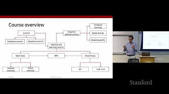
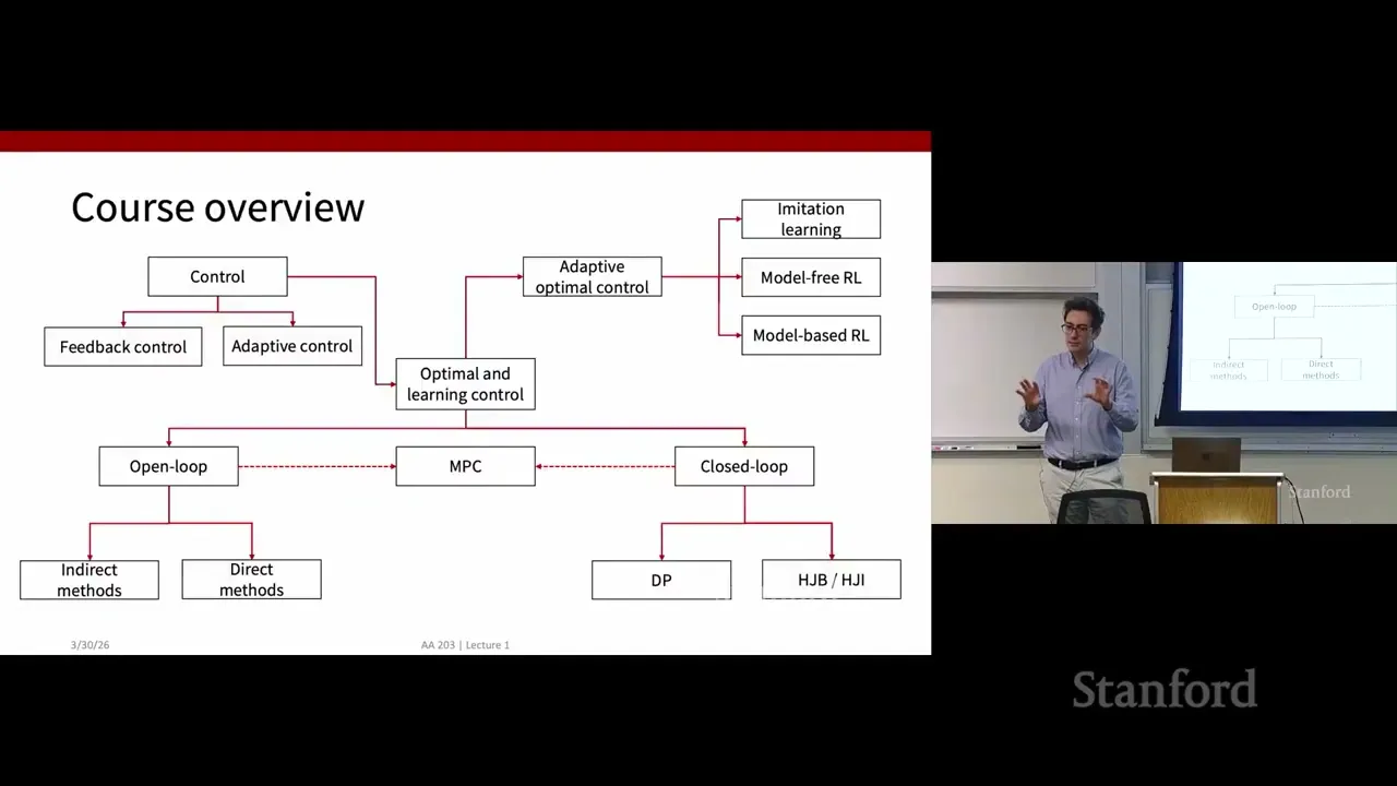
The instructor opens by orienting everyone to the class roadmap, so listeners understand what material sits behind them and what is coming next. Over the prior week, the class moved into the open‑loop optimal control quadrant of the roadmap. Last Monday they first touched on indirect methods, and this lecture continues deep diving into that same topic area.
 

Looking ahead: the following Wednesday lecture will shift over to direct open‑loop optimal control techniques. After finishing open‑loop material, the course will begin covering closed‑loop approaches in subsequent weeks.
 

One core mental model the lecturer keeps reinforcing is what indirect methods actually accomplish. Indirect methods give us necessary optimality conditions for infinite‑dimensional optimal‑control optimization problems. Infinite‑dimensional here means we are optimizing functionals. A functional takes a whole function as its input, rather than just a finite list of scalar numbers. Our target is to solve for an optimal control time history \(u^{*}(t)\), a continuous signal defined between an initial time \(t_0\) and final time \(t_f\).
 

This is not small tweak on finite‑dimensional calculus. We have to extend everything we know from standard finite‑variable optimization into this function‑space setting. That extension gives us the main building block: the fundamental theorem of calculus of variations.
 

I found one distinction here really helpful. In finite‑dimensional optimization, a local optimum requires the gradient equals zero. In this infinite‑dimensional variational setting, the analogous rule is that the first variation of the cost functional J must vanish at the optimal trajectory, for every valid admissible variation \(\delta x\). The lecturer draws this explicit parallel repeatedly, to keep students from treating variational calculus like some totally alien math.
 

Even though this vanishing‑variation rule tells us what an optimum must satisfy, it is not directly usable for computation. You cannot just plug numbers into that abstract condition. That is why the prior lecture worked through a simplified setup to turn this abstract necessary condition into something actionable.
 

That simplified problem assumed we could directly optimize the state trajectory itself. There was no separate explicit control input u. Both initial and final boundary conditions were fully fixed: initial time, final time, starting state, ending state all had hard given values. Starting from there, they expanded the functional’s increment, kept only its linear portion, and derived the Euler equation. The lecturer jokes they basically raced through Newton‑style derivation within a single lecture session.
 

The Euler Equation: Infinite‑Dimensional “Gradient Equals Zero”

 

The lecturer stresses you should think of the Euler equation as the infinite‑dimensional counterpart to the finite‑dimensional “gradient = zero” optimality check. Unlike the pure variation‑vanishing statement, the Euler equation produces a differential equation we can actually work with.
 

Important detail: this is a second‑order nonlinear ordinary differential equation. It also comes with split boundary conditions. This is where many learners hit friction. A standard initial‑value (Cauchy) problem gives you all required conditions only at the starting time, and you integrate forward. Split boundary conditions spread constraints across both the start and end time points of your time horizon. Mathematically solvable, but computationally trickier than simple forward integration from full initial states.
 

A brief student question pops up at around the 6‑minute mark. The student notes this whole derivation lives inside this simplified problem setup, where we pretend we directly command state trajectories, instead of computing optimal control sequences. The instructor confirms this limitation. The simplified case exists purely to build our mathematical toolbox. Upcoming slides will remove these simplifications and build toward real optimal‑control problems that include control inputs.
 

The lecturer announces they will walk through a concrete worked example, using the math they just reviewed. The example computes the shortest path connecting two separate points. It gives students hands‑on practice applying the Euler equation mechanics. After finishing this example, the lecture will start relaxing the fixed‑endpoint assumptions built into the simplified variational setup.
 

Worked Example: Shortest Path Between Two Points

 

The goal of this exercise is to use calculus of variations to prove the shortest path between two points is a straight line. Conceptually, we first need to write down a functional representing total path length.
 

From basic calculus, path length comes from summing infinitely tiny segment lengths ds. Using the Pythagorean theorem for infinitesimal time and position displacements, we write \(ds^2 = dt^2+dx^2\). Factoring out dt, we rewrite the infinitesimal segment as \(ds = dt\sqrt{1+\dot{x}(t)^2}\). Our cost functional J, total path length, becomes the definite integral from starting time \(t_0\) to final time \(t_f\) of that square‑root expression. Our integrand function \(g(x,\dot{x},t)=\sqrt{1+\dot{x}^2}\).
 

Next step: compute the partial derivatives required for the Euler equation. The integrand g has no dependence on x itself, only on \(\dot{x}\). So partial derivative of g with respect to x evaluates straight to zero. We then compute partial derivative with respect to \(\dot{x}\). After differentiation and simplifying algebra, the Euler condition reduces to an expression where \(\ddot{x}\) divided by a strictly positive term equals zero.
 

Since denominator is always positive, the only valid solution is \(\ddot{x}=0\). Integrating twice gives \(x(t)=c_1 t + c_2\), the formula for a straight line. We use our two fixed boundary conditions \(x(t_0)=x_0\), \(x(t_f)=x_f\) to solve for integration constants \(c_1\) and \(c_2\).
 

The lecturer makes a careful caveat here. What we have proven is that the straight line is a candidate for optimality. The necessary conditions do not, by themselves, guarantee global optimality. Second‑order analysis would be required to fully confirm this is truly the minimal‑length solution. Still, the example beautifully demonstrates step‑by‑step how you take a real‑world optimization question, cast it as a variational problem, apply Euler equation machinery, and recover an expected answer.
 

A quick classroom clarification moment happens near 17:25. A student misreads the double‑dot second derivative notation; the instructor and teaching assistant clarify the notation on the projector. It is a small moment, but highlights how easy it is to misinterpret derivative dots when following lecture live.
 

Relaxing Boundary‑Condition Constraints

 

Having wrapped up the shortest‑path example, the lecture moves toward material relevant for actual optimal‑control problems. The first big modification to our earlier formalism is relaxing our strict boundary‑condition rules.
 

Up to this point, every derivation assumed initial time \(t_0\), initial state \(x_0\), final time \(t_f\), final state \(x(t_f)\) were all fixed quantities. Now we allow final time and final state to be either fixed or free variables. Initial time and initial state remain fixed in this part of discussion.
 

The lecturer notes the core Euler differential equation itself still holds. The change does not alter the differential equation we solve. The problem we face: we lose some of our boundary constraints. Second‑order ODE requires two boundary values to pin down integration constants. If some final‑time quantities become free, we no longer have enough given conditions. We need new, replacement boundary conditions derived from optimality, these are called transversality conditions.
 

The lecturer says for today’s session they will mostly state these resulting conditions, rather than deriving them line‑by‑line. The algebraic manipulations are very repetitive, similar to the Monday lecture work, and do not offer huge new conceptual insight. Class time will focus instead on understanding what these conditions say and how to apply them.
 

These new conditions show up as an equation containing variations of final state \(\delta x_f\) and variations of final time \(\delta t_f\). How we handle the equation depends on which quantities are free versus fixed. If a variable is fixed, its admissible variation must equal zero, and that whole corresponding term vanishes. If a variable is free, the optimality condition forces the coefficient multiplying that variation term to equal zero.
 

Unanswered / Confusing Points Raised in Lecture

 

This section captures spots that felt under‑explained or left open by the lecturer, from my perspective as a listener.
 

First, transversality conditions get stated but not fully derived in this lecture. We learn the rule of thumb: fixed quantity → variation zero; free quantity → coefficient must vanish. But we do not walk through a full numerical example of a free final‑time or free‑final‑state problem. Seeing a small concrete example would make it easier to parse how to assemble boundary conditions for mixed fixed‑free endpoint scenarios. The lecturer signals this practical application work is likely coming in later course segments.
 

Second, the lecturer emphasizes that Euler equation delivers only necessary optimality conditions. Necessary means any true optimum has to satisfy these equations, but solutions to Euler equations might be maxima or saddle points instead of minima. The shortest‑path example waves at second‑order sufficiency checks but never demonstrates what that check looks like in a variational‑calculus context. It is easy for someone working homework to treat every Euler‑equation solution as automatically an optimal minimum, which is not guaranteed.
 

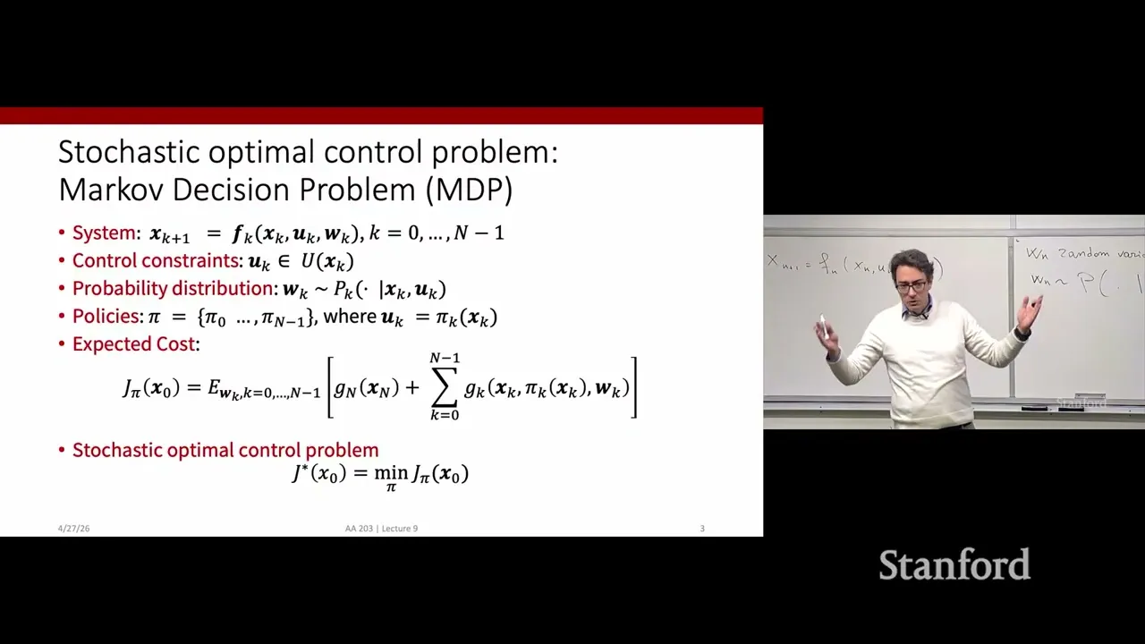
Third, the entire segment we watch stays within the indirect‑method simplified setting with no explicit control inputs. We see the math for state‑trajectory optimization, but we do not yet see how to map this variational machinery over to standard optimal‑control form with state dynamics \(\dot{x}=f(x,u)\). The instructor says future slides will bridge this gap, but at the end of this lecture chunk that connection is still pending.

Content Disclaimer: This article is for general reference only and does not constitute professional R&D guidance, production process advice or quality certification. All material performance data has specific test premises; readers should verify parameters against actual equipment and working conditions.