Stanford AA203 Optimal and Learning-Based Control | Spring 2026 | Lecture 10: Reachability Analysis — Annotated Lecture Notes & Key Takeaways

Course Information

Institution: Stanford

Original Course: Stanford AA203 Optimal and Learning-Based Control | Spring 2026 | Lecture 10: Reachability Analysis

Instructor Bio: Taught by Prof. Marco Pavone and Dr. Daniele Gammelli, with prominent work on safety verification and reachability analysis for autonomous systems.

Course Description: This lecture covers reachability analysis theory, including HJI equation derivation and state reachable set computation. It analyzes safety boundary verification under uncertainty, and introduces use cases in autonomous system validation.

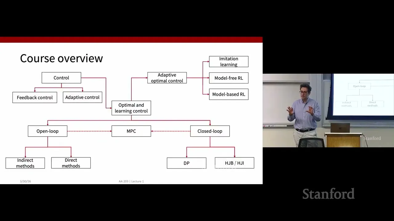
Lecture 10 of Stanford’s AA203 Optimal and Learning-Based Control course, themed around reachability analysis, opens with a quick, deadpan joke about restaurant diversity before diving into a substantial wrap-up of the prior class’s work on stochastic dynamic programming. Before getting to reachability-specific content, the lecturer spends the bulk of the transcribed segment reinforcing how to solve infinite-horizon Markov decision processes (MDPs). These solution methods — value iteration and policy iteration — form the foundational toolkit you need to make sense of closed-loop control and reachability problems later on. The lecture also teases future topics in learning-based control, where many of these same ideas get repurposed for settings where the system model is unknown.
 

Infinite-Horizon MDPs: Bellman Equations as Fixed-Point Problems

 

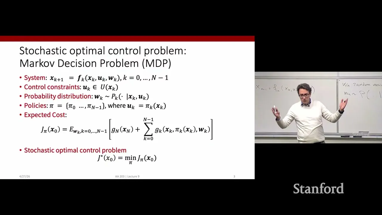
Picking up exactly where last lecture left off, the core goal here is extending stochastic dynamic programming from a finite time horizon to an infinite one. In finite-horizon problems, the value function changes at every time step as you count down to the end. In the infinite-horizon setting, by contrast, we’re looking for a stationary optimal value function that stays the same forever — it only depends on what state you’re in, not on what time it is.
 

The optimal value function, denoted V*(x), represents the maximum expected total discounted reward you can accumulate starting from state x if you act optimally for all future steps. It satisfies what’s called a fixed-point Bellman equation. Put simply, the optimal value at any state equals the maximum over all possible control actions of two things: the immediate reward you get for taking that action, plus the discounted expected optimal value of whatever state you end up in next.
 

The lecturer also walks through the Q-function, a related quantity that takes both a state and an action as inputs. The optimal Q-function Q*(x,u) captures the total reward you get for starting in state x, taking action u, and then acting optimally for every step after that. It follows a nearly identical fixed-point structure to the value function. The lecturer notes Q-functions become especially useful in learning settings, though we won’t dive deep into that for another three or four lectures.
 

One small convention note worth flagging: the entire lecture frames everything in terms of reward maximization, not cost minimization. If you’ve been working mostly with cost-based control formulations lately, this flip can take a second to adjust to. Higher values mean better performance here, and we take maxima instead of minima at each decision point.
 

For any fixed policy π — that is, a rule that tells you exactly what action to take in each state — you can also compute its value function V_π(x), which is the expected reward you get if you follow that policy forever. In a finite state space, this is just a vector with one entry per state, and solving for it amounts to solving a linear system of equations. That fact becomes important when we get to policy iteration.
 

Value Iteration: Iterative Backup to Optimal Value

 

Once the Bellman equation is defined as a fixed-point problem, the obvious practical question comes up: how do we actually solve it? We know the reward function and we know the transition probabilities between states, but we don’t know the optimal value function or the optimal policy.
 

The lecturer explains there are two broad categories of algorithms for the known-model setting. The first is value iteration.
 

The core idea is very intuitive. You start with some initial guess for the value function. The simplest possible guess is just setting the value of every state to zero. Then you repeatedly apply the Bellman backup formula, updating your entire value function estimate each iteration, and you keep doing that until the values stop changing much.
 

It turns out this algorithm is mathematically guaranteed to converge to the true optimal value function, no matter what initial guess you start with. If you start with a reasonably good guess, convergence is much faster. If you start with all zeros, it just takes a few more iterations. There’s no risk of diverging or getting stuck on a wrong answer.
 

The lecturer uses a helpful analogy to build intuition for why this works. Imagine you take an infinite-horizon problem and approximate it as a finite-horizon problem with an absurdly long time horizon — say, three trillion years. You start at the very end with zero value, then do standard backward induction step by step, working your way all the way back to the present day. Do that enough times, and you’ve effectively approximated the infinite-horizon solution. A student asks if this is really just dynamic programming for an extremely long horizon, and the lecturer confirms that’s exactly the underlying intuition.
 

What’s less satisfying is how you know when to stop. There’s no universal, one-size-fits-all answer. Common practical rules of thumb include stopping when the maximum difference between value estimates across all states drops below some small threshold, or just running a fixed number of iterations — the lecturer throws out 20,000 as an offhand example — and calling it a day. More sophisticated mathematical methods can give you formal error bounds on how close you are to the true optimal value, but those are more advanced and not covered here. For most practical purposes, people use simple heuristic stopping criteria.
 

The same basic approach works for Q-functions too. Instead of iterating on the value function V, you iterate on the Q-function fixed-point equation, following exactly the same logic.
 

Policy Iteration: Improving Policies Directly

 

The second major algorithm for known-model MDPs is policy iteration, which takes a fundamentally different approach. Instead of iterating on the value function and then extracting an optimal policy at the very end, policy iteration works directly in the space of policies. It alternates between evaluating how good a given policy is and using that information to make the policy better.
 

Each full iteration of the algorithm has two steps.
 

First is policy evaluation. Given your current candidate policy π_k, you calculate its value function V_πk. Because you’re not trying to maximize over actions — you just use whatever action the policy prescribes in each state — this is not an optimization problem. It’s just a linear system of equations with one unknown per state. For a problem with 10 states, you have 10 unknown values and 10 equations, so you can solve it with standard linear algebra.
 

Second is policy improvement. You take the value function you just computed for the current policy and use it as a surrogate for the true optimal value function. Then, for each state, you pick the action that maximizes the immediate reward plus the expected discounted future value. This gives you a new, updated policy π_{k+1}.
 

The key theoretical result here is that the new policy is always at least as good as the old one. If the old policy was not already optimal, the new policy is strictly better. The lecturer calls this the monotonic improvement property, and notes that full proofs are available in standard dynamic programming textbooks, citing Bertsekas as a standard reference.
 

Because there are only a finite number of possible policies when you have a finite number of states and a finite number of actions, policy iteration is guaranteed to converge in a finite number of steps. That’s a notable difference from value iteration, which converges asymptotically but never technically reaches the exact optimal value in finite steps.
 

A student asks early on if there’s any way to know in advance how many iterations you’ll need. The lecturer uses this question to tee up policy iteration’s finite convergence as a key advantage, though they note that each iteration is more computationally expensive because of the linear system solve.
 

Unfinished Threads and Reachability Context

This is where the transcribed segment shows its edges, and where we can ground all this MDP material back to the lecture’s stated focus on reachability analysis.
 

First, the transcript cuts off mid-sentence right as the lecturer is drawing a comparison between value iteration and policy iteration. We get the basic structure of each algorithm and their core convergence properties, but we don’t get the full breakdown of practical tradeoffs: when you should pick one over the other, how their runtimes scale with state space size, or common implementation pitfalls. From what’s implied, policy iteration often converges in fewer iterations but each step is heavier, while value iteration has cheap iterations but tends to need more of them. We don’t get the lecturer’s full on-the-record take.
 

I also found the Q-function section a bit underdeveloped. We’re told repeatedly that Q-functions are important for learning settings, but there’s no concrete example of why that is, or how they connect to the reachability analysis the lecture is named for. It feels like setup for future material without much payoff in this segment.
 

Most notably, the lecture’s titular topic — reachability analysis — is only referenced as the broader context for all this foundational material. The transcribed portion stays almost entirely on MDP solution methods, with the opening promise of moving on to closed-loop optimal control and reachability after the recap. For anyone who showed up specifically to learn about reachability, this part of the lecture is almost all prerequisite setup.
 

That said, the connection is logical even if it’s implicit. To analyze whether a stochastic system can reach a desired set of states under optimal closed-loop control, you first need to know how to compute optimal policies and value functions. These MDP algorithms are exactly the tools that make reachability calculations tractable for systems with uncertainty. You can think of reachability as asking “can we get there?” and these dynamic programming methods as answering “what’s the best way to try?”
 

While this segment of the lecture focuses heavily on dynamic programming fundamentals, it lays essential groundwork for understanding reachability analysis in controlled stochastic systems. Value iteration and policy iteration aren’t just abstract MDP solvers — they’re the computational backbone for determining what controls will drive a system toward target states, which is the core question of reachability. Missing details and cut-off explanations aside, this lecture does a solid job refreshing the algorithmic toolkit you’ll need to tackle that analysis.

Content Disclaimer: This article is for general reference only and does not constitute professional R&D guidance, production process advice or quality certification. All material performance data has specific test premises; readers should verify parameters against actual equipment and working conditions.