Stanford AA203 Optimal and Learning-Based Control ｜ Spring 2026 ｜ Lecture 16： Fundamentals of RL — Annotated Lecture Notes & Key Takeaways

Course Information

Institution: Stanford

Original Course: Stanford AA203 Optimal and Learning-Based Control ｜ Spring 2026 ｜ Lecture 16： Fundamentals of RL

Instructor Bio: Taught by Prof. Marco Pavone and Dr. Daniele Gammelli. Reinforcement learning fundamentals are a core module of the AA203 curriculum.

Course Description: This lecture breaks down RL fundamentals. It introduces Markov Decision Processes, reward functions and policy optimization goals, explains basic policy gradient algorithms like REINFORCE, and discusses core challenges such as high variance.

This is Lecture 16 of Stanford's AA203 Optimal and Learning-Based Control course, Spring 2026, and it marks a major turning point in the syllabus. After spending the previous session on imitation learning, the instructor pivots fully into reinforcement learning — the paradigm that will anchor the rest of the course. The lecture mixes recap, formal foundations, a concrete worked example, and a preview of what's next, with a few quick Q&A asides that clarify common points of confusion.
 

From imitation learning to reinforcement learning: why the shift?

 

Last week covered imitation learning — learning control policies directly from expert demonstrations. The two main approaches were behavioral cloning (mimicking the expert's actions directly) and inverse reinforcement learning (inferring the reward function the expert is optimizing). The instructor emphasizes a hard ceiling here: no matter how well you implement imitation learning, your performance can never exceed the quality of the demonstrations you're learning from. You're capped at the expert's level.
 

That's the core motivation for moving to reinforcement learning. Instead of learning from demos, RL agents learn by interacting with their environment through trial and error. They don't just copy someone else's solution — they discover their own, which can potentially surpass any given expert.
 

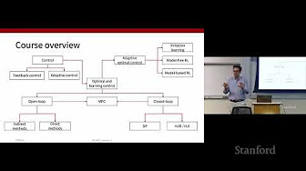
The roadmap for the next few lectures: the next two sessions will focus on model-free reinforcement learning, followed by model-based RL. Today's lecture is mostly setup — a recap of the RL problem formulation, a deep dive into "exact" solution methods rooted in dynamic programming, and a first look at two fundamental model-free approaches: Monte Carlo learning and temporal difference learning.
 

MDP foundations and the Bellman equation toolkit

 

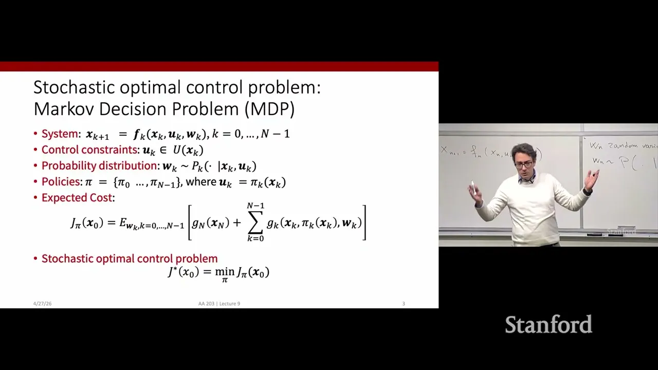
RL problems are formalized using Markov Decision Processes, or MDPs. The instructor frames an MDP as a five-part mathematical object: a state space (all possible situations the agent can be in), an action space (all possible moves the agent can make), a transition function (the probability of landing in each next state, given a current state and action), a reward function (a scalar score for each state-action pair), and a discount factor between 0 and 1.
 

The discount factor serves two purposes. Intuitively, it weights immediate rewards more heavily than far-future ones, which matches how most real-world decisions work. Mathematically, it turns an infinite sum of future rewards into a finite, calculable value.
 

The goal of RL is straightforward on paper: find the optimal policy π* — a rule for picking actions in every state — that maximizes the expected total discounted reward over time.
 

To talk about how to find that policy, the instructor recaps two core functions. The state value function V^π(s) tells you the expected total reward starting from state s and following policy π forever after. The action-value function Q^π(s,a) is similar, but starts from state s, takes action a once, then follows policy π.
 

Both satisfy fixed-point relationships called Bellman equations. There's the Bellman optimality equation for the optimal value functions V* and Q*, and the Bellman expectation equation for any arbitrary policy. The Q function is particularly useful in practice, the instructor notes, because you can extract a policy directly from it — just pick the action with the highest Q value in each state, no extra planning step required.
 

In tabular form (finite, enumerable states and actions), V is a list of numbers, one per state, and Q is a matrix with a row for every state and a column for every action.
 

Exact solution methods: value iteration and policy iteration

 

The instructor refers to dynamic programming-based methods as "exact methods" because, when they converge, they give the mathematically optimal value function and policy. The catch: they only work if you already know the full transition dynamics — the exact probability distribution of next states for every state-action pair.
 

Two standard algorithms here. Value iteration works by repeatedly applying the Bellman optimality equation to your estimate of V, updating every state's value based on the best possible action and the expected value of the next state. Keep going until the value function stops changing by more than some tiny threshold.
 

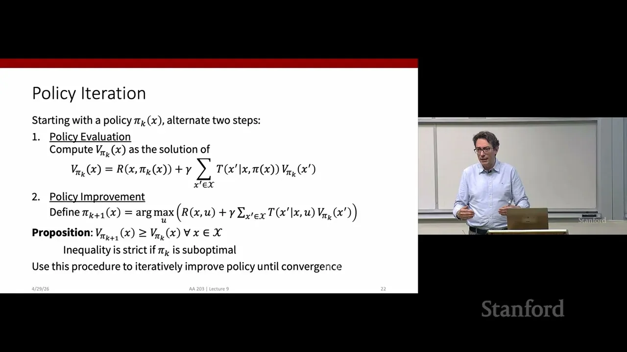
Policy iteration takes a two-step cycle. First, policy evaluation: given your current policy, compute its corresponding value function by enforcing the Bellman expectation equation until convergence. Second, policy improvement: use that value function to make a better policy by acting greedily — picking whichever action leads to the highest expected value. Then go back to evaluation with the new policy, and repeat until the policy stops changing.
 

Both algorithms are proven to converge to the optimal solution for finite MDPs. The catch, which the instructor circles back to multiple times, is that both rely entirely on knowing the system's dynamics. In most real control problems, you don't have that information up front.
 

Policy iteration walkthrough: a grid world example

 

To make policy iteration less abstract, the instructor walks through a classic grid world example. It's a 4×4 grid — 16 cells total. Fourteen are regular non-terminal states, and two are terminal goal states. The agent can move up, down, left, or right; if a move would take it off the edge, it just stays in place.
 

The reward structure is simple: every step gives -1 reward, and there's no extra reward for reaching the goal. This naturally encourages the agent to reach a terminal state as quickly as possible, since every extra step costs you. For simplicity, the discount factor γ is set to 1 — no discounting of future rewards.
 

The instructor starts with the most basic initialization possible: a completely random policy (each action has 25% probability in every state) and a value function initialized to all zeros.
 

Walking through the first policy evaluation iteration: every non-terminal state gets updated to -1. That's because you take one step, get -1 reward, and all the next states still have value 0 from the initial guess. As more evaluation iterations run, values propagate backward from the goal states — cells closer to the goal have less negative values, since fewer steps are needed to get there.
 

Once evaluation converges (or even after a few steps in simple cases), you do the policy improvement step. For each state, look at all four neighboring cells and pick the action that moves toward the one with the highest value. Visually, this gives a grid of arrows all pointing toward the nearest goal — exactly what you'd expect the optimal policy to look like.
 

A student asks about initialization: is all zeros just a convention? The instructor says yes, it's a default for when you have no prior information. If you do have a rough idea of what good state values should be, plugging those in can speed up convergence significantly.
 

Another student asks about termination criteria — how do you know when to stop? The instructor explains that policy iteration is proven to converge in finite state spaces, so running it long enough guarantees the optimal policy. In practice, people use rules like stopping when the value function changes by less than some small delta, or when the policy stops changing between iterations. There's no single universal best rule.
 

I found this part a little hand-wavy. A concrete comparison of how different termination criteria affect speed versus solution quality — especially for larger problems — would have helped.
 

Why exact methods aren't enough: the case for model-free RL

 

This is the punchline of the lecture, and the reason we're moving into reinforcement learning proper. Every exact method covered so far — value iteration, policy iteration, all the dynamic programming machinery — requires perfect, complete knowledge of how the environment works. You need to know exactly what happens when you take every action in every state.
 

In almost any interesting real-world control problem, you don't have that. There's no pre-written transition function. You have to take actions, observe what happens, and learn from the results.
 

That's the core of reinforcement learning as a paradigm: learning from interaction. And that's what the next set of methods — model-free RL — are designed for. The lecture ends by teeing up two foundational model-free approaches: Monte Carlo learning, which learns from full episodes of experience, and temporal difference learning, which updates estimates after every single step.
 

The instructor doesn't dive deep into either one yet, but frames them as natural extensions of the value estimation ideas already covered — just without the transition model.
 

Overall, this lecture doesn't just recap RL basics — it builds a logical bridge from the controlled, known-world dynamic programming solutions to the messy, interactive learning problem that defines RL at its core. By the end, you can see exactly why exact methods are powerful but limited, and why model-free reinforcement learning is necessary for tackling real-world control problems where the dynamics are unknown.

Content Disclaimer: This article is for general reference only and does not constitute professional R&D guidance, production process advice or quality certification. All material performance data has specific test premises; readers should verify parameters against actual equipment and working conditions.