Stanford CS221 | Autumn 2025 | Lecture 6: Search II — Annotated Lecture Notes & Key Takeaways

Course Information

Institution: Stanford

Original Course: Stanford CS221 | Autumn 2025 | Lecture 6: Search II

Instructor Bio: This lecture is delivered by Percy Liang, Associate Professor of Computer Science at Stanford University and core faculty of the Stanford Institute for Human-Centered Artificial Intelligence (HAI). Percy Liang leads the Stanford Natural Language Processing Group and the Center for Research on Foundation Models (CRFM). His research spans the theoretical foundations and practical systems of artificial intelligence, including machine learning, natural language processing, AI alignment, and rigorous model evaluation. He received his PhD in Computer Science from the University of California, Berkeley and his BA in Mathematics from Harvard University. His work has been recognized with the NSF CAREER Award, Google Faculty Research Award, and multiple best paper awards at top-tier AI conferences. He has taught CS 221 at Stanford for over a decade, shaping foundational AI education for thousands of students.

Course Description: This second search lecture covers informed and heuristic search strategies that leverage domain knowledge to guide exploration efficiently. It focuses on A* search, its admissibility conditions, heuristic design principles, and optimizations for reducing search complexity. The lecture also explores local search algorithms including hill climbing, simulated annealing, and genetic algorithms for solving optimization problems where systematic state-space exploration is computationally infeasible.

Percy Liang spends this lecture finishing the story that Lecture 5 started: how to do exact search​ when the state graph is allowed to have cycles. That single relaxation of the assumptions forces a redesign of the whole algorithm, and the two things that come out of it — uniform cost search and A* — turn out to be the same algorithm wearing different clothes. If you only have time for one idea, it's the second half: the heuristic trick that makes A* work is a change of edge costs, not a change of algorithm.
 

Two housekeeping notes before anything else. The auto-captioning on the recording is rough, and it consistently mangles the technical vocabulary: "AAR" is A*, "Dystra" is Dijkstra, "heristic" is heuristic, "pass cost" is past cost, "emissibility" is admissibility, "Markoff" is Markov. I've silently corrected all of these below. The lecture is also heavily demo-driven — he runs code live on two or three toy problems — so some of the value is in watching the frontier grow, which doesn't survive in prose. I've noted where that happens.
 

Why cycles break the dynamic programming we already had

 

The first few minutes are a recap. A search problem is a start state, a successor function giving you actions out of each state, a cost per action, a test for whether you've hit an end state, and the goal of minimizing the sum of action costs. The running example from the previous lecture is a tram problem: six locations, you can walk or take a tram, get from 1 to 6 as cheaply as possible. Lecture 5 covered four algorithms — exhaustive search, dynamic programming (which he describes as exhaustive search with a cache), best-of-n sampling, and beam search — with the first two framed as exact methods that compute a future cost for every state.
 

Then he introduces the mirror concept. Future cost answers "from here, what's the cheapest way to reach an end state." Past cost answers "what's the cheapest way to get from the start to here." Every state has both, and past cost plus future cost gives you the cost of the best complete solution that routes through that state. It's a genuinely useful mental image, and he asks for it explicitly: stand at a state, look backward for one quantity and forward for the other.
 

The trouble is directional. Future cost of a state is defined in terms of the future costs of its successors, so to compute it you must already have computed the successors. In a graph with no cycles, that's fine — you get a topological ordering, fill the cache from the end backward, and stop when you reach the start. He draws an analogy to backpropagation here: written as a recurrence, executed backward from the end. The connection is real but he only gestures at it, and I would have liked more than "there's a deeper connection here."
 

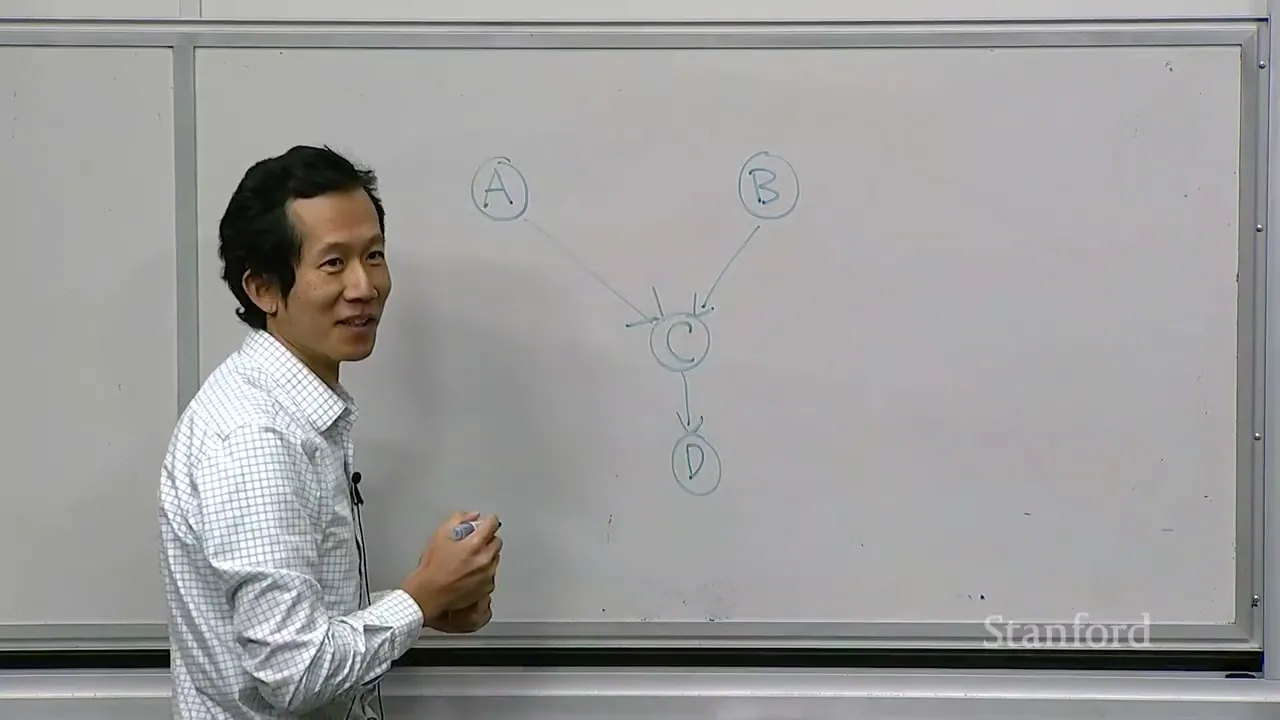
Add cycles and the whole thing collapses. A student in the room gives the answer he's fishing for: in code you get an infinite loop, and mathematically the quantity simply isn't defined, because the future cost of state s would depend on the future cost of s′ while s′ depends back on s. His concrete example is a four-node undirected graph — A–B costs 1, A–C costs 100, B–C costs 1, B–D costs 100, C–D costs 1, symmetric in both directions. Which node do you evaluate first? There is no ordering to lean on (2:22 onward), and the "obvious answer" of uniform cost search is, by his own admission, not yet motivated.
 

Uniform cost search: ordering states by cost instead of by topology

 

Uniform cost search — Dijkstra's algorithm, developed in the 1950s — makes an explicit trade. It gives up the acyclic requirement, and in exchange demands that every action cost be non-negative. Negative edges plus cycles are handled by Bellman-Ford, which he names, notes he won't cover, and moves on from in about four seconds.
 

Two changes relative to dynamic programming. First, compute past costs instead of future costs. Second, and this is the part he flags as the key insight, process states in increasing order of past cost. Where dynamic programming borrowed an ordering from the graph's structure, UCS manufactures its own ordering from the numbers it is computing. That self-reference is what makes cycles survivable, and it's also why the proof later on has to work a little.
 

Mechanically, states get partitioned into three buckets: explored (we've locked in the cheapest path here), frontier (we've seen it, but a better route might still turn up), and unexplored. The frontier is a priority queue whose priority for each state is the cheapest cost found so far. Each entry also carries a back pointer recording the previous state and the action taken — not needed if you only want the cost number, but necessary if you want the actual solution, which you usually do.
 

The worked example is the four-node graph above, and it's worth walking through once because it's where the frontier-update logic clicks. Pop A at cost 0. Push B at 1 and C at 100. Pop B at 1; A is already explored so the back edge is skipped; C is already on the frontier at 100 but B offers a route at 2, so C's priority is decreased and its back pointer reassigned from A to B; D is new and joins the frontier at 101. Pop C at 2; A and B are explored, and D can be reached at 3, so D drops from 101 to 3. Pop D. D is an end state, so stop and follow the back pointers home: A→B→C→D, total cost 3.
 

What I appreciate about this example is that it hides nothing. Things on the frontier are states you've visited, not states you've solved — he says this outright — and the same node can be reprioritized multiple times. The 100 on the A–C edge exists purely to make the point that a greedy first impression gets corrected later.
 

He then runs a 5×5 grid — move up/down/left/right, cost 1 each, walls marked, start at (0,0), end at (4,4) — and gets an optimal cost of 14, and follows it with a video of UCS on a much larger grid where each pixel is a state. Explored states are one color, the frontier another, unexplored a third, with a green trace showing the path back from whichever frontier node is being popped. This is the moment the name lands: the search blossoms outward uniformly from the start, because it has no idea where the end is. It will get there if the graph is connected. It'll also waste an enormous amount of effort going the wrong way, and he explicitly draws your attention to that waste because it's the setup for everything after.
 

Then comes the correctness argument (around 22:17). The claim: whenever UCS moves a state from the frontier to explored, its priority equals its true past cost. Prove that and you're done, because it holds in particular for an end state. The proof is by induction over pops. Base case is the start state at zero. For the inductive step, take the path the algorithm actually found (he calls it the blue path, with cost equal to the priority) and any rival path (the red path). The red path must cross from the explored region into the unexplored region at some edge from a state t to a state u. Bound the red path from below: the cost of getting to t is at least the past cost of t; by the inductive hypothesis that equals the priority of t; when t was explored, the algorithm would have offered u a priority of at most priority(t) plus the t→u edge cost; and u is at least as expensive as s, since s was the one popped. The remaining tail from u to s can be discarded because costs are non-negative — and that's precisely where non-negativity is load-bearing. He gives the intuition separately and I found it more convincing than the algebra: with negative edges you could wander off, collect a huge negative cost, and come back cheaper than the route UCS already committed to.
 

A* is uniform cost search in a heuristic costume

 

The pitch for A* is the video from before, run again (31:13). UCS spreads in all directions; a large fraction of it is obviously wasted. What we want is to order exploration by past cost plus future cost, which would keep us on an optimal path the whole way. We can't, because the future cost of the start state is the answer to the problem. So approximate it: a heuristic h(s), a function from states to numbers that estimates remaining cost.
 

Here's the move I did not see coming, and it's the intellectual center of the lecture. A* isn't a new algorithm at all. It's UCS run on a modified search problem where every edge cost becomes:
 

c(s, a) + h(s′) − h(s)
 

That is, you take the real cost and add a term that rewards you for moving closer to the goal and penalizes you for moving away. If h is a good estimate of remaining distance, then moving toward the end makes the bracket negative and the modified edge cheap.
 

The demonstration is a line: integer states, start at 0, end at 2, every move costs 1. UCS expands outward symmetrically in both directions and eventually finds the goal. Define h(s) = 2 − s, so h is 2 at the start, 0 at the end, 3 at −1. Going right then costs 1 + 1 − 2 = 0. Going left costs 1 + 3 − 2 = 2. Suddenly the modified problem has a free edge to the right and an expensive edge to the left, and UCS walks straight to the goal. The one bit of bookkeeping: the returned path has modified costs of zero, which isn't what you wanted, so you walk the steps and undo the h(s′) − h(s) term on each one to recover original costs. He's candid that this is clerical work, and it's the kind of thing that would bite you in an implementation.
 

A student asks the question that drives the next ten minutes: can that subtraction produce a negative modified cost? Yes, and he has an example ready — heuristic values in red, original edge costs in blue, modified costs in purple, one of which comes out to −9999, which UCS won't even accept. The heuristic in that example isn't merely inaccurate, it's close to adversarial, steering the search away from the good branch. So the condition for A* to be legal is exactly what you'd guess: all modified edge costs must be non-negative. That property has a name — consistency — plus the trivial requirement that h be zero at an end state, since remaining cost at the goal is zero by definition.
 

He is mildly sheepish about the circularity of this, joking that it's almost too convenient: someone asks what happens if modified edges go negative, and the answer is "then don't let them." Fair, but I'd push back slightly — "modified edges are non-negative" is a condition on a derived quantity, and if you just wrote down a heuristic on the back of an envelope you'd have to check it on every edge of your graph. He acknowledges this is hard to check directly, and the entire second half of the lecture is really the answer to that worry.
 

The correctness proof is short and elegant. Take any path from start to end. Each modified edge contributes its original cost plus an h(s′) − h(s) term. Sum the whole path and those terms telescope: you add h at the second state and subtract it, add it at the third and subtract it, and the final h is zero at the end state. What survives is the original path cost minus h(start). Since h(start) is the same constant for every path, minimizing modified cost and minimizing original cost select exactly the same paths (46:21). The intuition he offers is nicer than the algebra: yes, you've perturbed every edge, but you've perturbed them in a coordinated way that undoes itself as you travel.
 

Does it actually help? He can't give a general bound, because it depends on the heuristic, but the comparison is clean. UCS expands every state whose past cost is at most the cost of the best end state. A* expands states satisfying the same inequality with the heuristic term subtracted, which is a strictly tighter condition. Set h to zero everywhere and A* degenerates into UCS. Set h to the true future cost and A* touches only nodes on an optimal path — wonderful, except that computing the true future cost is the original problem. Real heuristics live between those extremes, and designing them is about buying the most leverage per unit of effort while staying consistent. He also mentions admissibility in a single breath — h never overestimates future cost, consistency implies it, it suffices for tree search but not graph search — then tells the class they can ignore it. I think that's the right call for lecture time and the wrong call for anyone who'll meet A* again elsewhere.
 

Getting heuristics for free by relaxing the problem

 

If consistency is hard to verify, the workaround is to construct heuristics that are consistent by design. The construction is relaxation (around 57:36): throw away some constraints of your original problem, compute the future cost of that easier problem, and use it as your heuristic. If you could compute the true future cost, it would certainly be consistent — but that's the original problem again. So compute the future cost of something adjacent that you can actually solve.
 

He gives three flavors, and they're the most practically useful part of the lecture.
 

Closed form.​ The 5×5 grid again. What's in the way? The walls. Delete them and the answer is just the Manhattan distance to the goal — start (0,0), end (4,4), so 8. No search required. He walks around the grid evaluating it: one state scores 2 because it looks two steps from the goal, but it's actually much farther because a wall forces you around; another looks distant but is genuinely close. The heuristic isn't perfect, and it doesn't need to be. It's the true future cost of a different problem, which is what buys consistency.
 

Fewer states.​ The tram problem from Lecture 5, in its limited form: you can walk one step or tram to double your position, but only as many times as you have tickets. Tracking tickets multiplies the state count by the number of locations times the number of tickets, and every search algorithm scales in state count. Relax it by making the tram free — no ticket bookkeeping — and the state is just the location. Solve that smaller problem with dynamic programming, then, when you need a heuristic value for an original state, project the state down by dropping the ticket component. On his instance UCS explored 23 states, A* explored 8. He's careful about the accounting and I respect it: you also paid 10 states to solve the relaxed problem, so the honest total is 18 against 23. Still better, much less impressive than the raw 8 suggests. A student calls him on precisely this and he concedes the point directly.
 

Independent subproblems.​ A sliding tile puzzle with one hole, where a move swaps an adjacent tile into the hole. In the real problem tiles can't overlap. Relax that and tiles pass through each other, which splits the puzzle into eight independent single-tile problems — each solvable in closed form by counting how far its tile has to travel. Sum them and you have your heuristic. He generalizes: whenever your state is a collection of objects with coupling constraints, deleting the coupling often factorizes the problem.
 

The unifying framing is slightly strange and I liked it. A constraint is just an infinite cost. Walking into a wall isn't forbidden, it costs infinity; relaxing means lowering that infinity to a finite number. So a relaxation, formally, is a problem with identical states, actions and successors, where costs are reduced or left alone — sometimes infinity down to finite, sometimes finite down to smaller finite. The three-line proof that such a heuristic is consistent is the triangle inequality: h(s) ≤ c(s,a) + h(s′), and since relaxed costs are no larger than original costs, that upper bound holds for the original costs too, which is exactly the consistency condition.
 

Two footnotes. If you have two consistent heuristics, take their pointwise maximum — also consistent, proof skipped as straightforward, which is a shame because it's the kind of thing that feels like it should be false. And if your relaxed problem has cycles you can't use dynamic programming on it, so reverse it: flip every edge, run UCS on the reversed problem, and the past costs you get are the future costs of the thing you wanted. He sketches this and sends it to homework.
 

Where the argument felt thin

 

Three things didn't fully land for me. The efficiency discussion is the weakest part of an otherwise tight lecture — there's no complexity statement anywhere, the 23-versus-18 comparison is a single hand-computed instance, and he says outright that whether relaxation pays off is an empirical question depending on how many states you save and how tight the bound is. True, but it leaves you with no guidance for deciding in advance.
 

Second, the grid demo. He runs the search, gets a cost of 8, and then says he's not sure why he ran it on the relaxed problem rather than the original and he'll fix it later. If you're watching the recording, the number on screen is the relaxed answer, not the A* answer, and it's easy to come away confused. He also concedes A* doesn't buy much on that grid anyway, since the problem is barely harder than linear in the number of states.
 

Third, the consistency criterion is defined as "whatever makes UCS applicable," and the lecture never quite closes the loop on verification: relaxation tells you how to build consistent heuristics, not how to test one someone handed you. A student also pointed out mid-lecture that the proof he'd just presented wasn't in the GitHub version of the notes yet, and he promised to fix it after class. Worth knowing if you're following along with the posted materials.
 

What to take away before Lecture 7

 

Uniform cost search and A* are both exact, both tolerate cycles, and both demand non-negative costs — that's the trade. They both work by expanding states in increasing order of cost, real cost for one and heuristically adjusted cost for the other, and the entire difference between them lives in a single line of arithmetic on the edge weights. Heuristics are best understood not as guesses but as the true future cost of an easier problem you chose on purpose.
 

The last thirty seconds point forward (1:19:31): next time actions stop being deterministic. Roll a die and "minimum cost" stops meaning what it used to, and the class moves to Markov decision processes and policies. Given how much this lecture leaned on the past-cost/future-cost distinction, I'd guess that pairing shows up again there.
 

Content Disclaimer:

This article is for general reference only and does not constitute professional R&D guidance, production process advice or quality certification. All material performance data has specific test premises; readers should verify parameters against actual equipment and working conditions.