Stanford CS221 |Lecture 2： Learning I.en_Transcript — Annotated Lecture Notes & Key Takeaways

Course Information

Institution: Stanford

Original Course: Stanford CS221 | Autumn 2025 | Lecture 2: Learning I

Instructor Bio: This lecture is delivered by Percy Liang, Associate Professor of Computer Science at Stanford University and core faculty of the Stanford Institute for Human-Centered Artificial Intelligence (HAI). Percy Liang leads the Stanford Natural Language Processing Group and the Center for Research on Foundation Models (CRFM). His research spans the theoretical foundations and practical systems of artificial intelligence, including machine learning, natural language processing, AI alignment, and rigorous model evaluation. He received his PhD in Computer Science from the University of California, Berkeley and his BA in Mathematics from Harvard University. His work has been recognized with the NSF CAREER Award, Google Faculty Research Award, and multiple best paper awards at top-tier AI conferences. He has taught CS 221 at Stanford for over a decade, shaping foundational AI education for thousands of students.

Course Description: This lecture opens the machine learning module of the course, introducing the core problem of supervised learning from labeled examples. It covers the fundamental formulation of empirical risk minimization, the linear regression model, and the ordinary least squares solution. The lecture also explains key conceptual pillars including loss functions, generalization, overfitting and underfitting, and the bias-variance tradeoff that defines the central challenge of statistical learning.

If you missed this one, the shape of it is: about twenty minutes finishing a topic from the previous class that the instructor felt he'd rushed, then the headline material — gradients, backpropagation, and a first pass at linear regression. He announces that plan at (0:08) and mostly sticks to it, though the detour through einsum eats more time than I think he expected.
 

Worth knowing up front: he opens by admitting he went through the tensor-notation library too fast last time and wants to slow down. That sets the tone for the hour. This is a lecture that keeps stopping to check whether people are following, and twice a student question derails it in a genuinely useful way.
 

Tensors, Named Axes, and einsum as the One Operation to Rule Them All

 

The framing is that tensors are the atoms of modern machine learning. Data, parameters, intermediate computations — everything is a tensor.
 

One small vocabulary decision he makes deliberately: he says "order" rather than "rank," because rank already means something different for matrices. Order zero is a scalar, order one a vector, order two a matrix, and he reminds us they'd already seen order four and order five tensors. A tensor of order n has n axes, and for a matrix, axis 0 is rows and axis 1 is columns.
 

The library under discussion — transcribed variously as "inops," "Ein sum," and "Einstein," but it's clearly einops plus einsum — does two things. First, you name your axes. His analogy for how: it's like naming variables in code. The program runs whether you call a thing strawberry or x, so pick the name that says what the axis represents. A data matrix whose rows are data points and whose columns are features gets axes named something like example and feature.
 

Second, einsum is presented as a kind of master operation. Last lecture it was introduced as a generalization of matrix multiplication; here he pushes it further, as a meta-operation that swallows dot products, sums, elementwise products, transposes, and matrix products as special cases.
 

The notation works like this. You write a string with input axis names to the left of an arrow and output axis names to the right; commas separate multiple input tensors. What appears on the right determines the order of the result. He walks through examples at a deliberately slow pace:
 

• Identity​ — i->i. Boring on purpose, to show the routing.
• Sum​ — i-> with an empty output. The result is order zero, a bare number, and everything gets dumped into it. His running vector (0, 1, 10) sums to 11.
• Elementwise product​ — i,i->i. Pass two tensors, multiply entry by entry.
• Dot product​ — i,i->, empty output again. He notes the point that dot product, sum, and elementwise product feel like distinct operations in a normal linear algebra course, and here they're the same machinery with different axis bookkeeping.
• Outer product​ — i,j->ij. The first example with two indices.

 

At (8:45) he takes a small detour that I think is the real argument for the whole notation: there are no transposes anywhere. He confesses that transposes personally confuse him, all that mental gymnastics about which symbol is the row and which is the column, and that with named axes you can look at the string and immediately see what's input and what's output. That's a claim about legibility, not power — and he seems more invested in it than in anything else in this segment.
 

He then goes a bit wild on purpose: i,i,i->i for an elementwise cube, i,j,k->ijk for a triple outer product producing an order-three tensor. He explicitly calls this "sort of useless," which is refreshing. It's there to show the notation can be pushed, not because you'd want to.
 

Then matrices: sum all entries, row sums, column sums, transpose as ij->ji, matrix-vector products, and two flavors of matrix-matrix product. The interesting case is the MᵀM form, where an index appears in the inputs but not in the output. When that happens, a given output cell receives contributions for every value of the summed-out index, and they accumulate. He's careful to spell out that this is literally what "sum out" means.
 

The general rule, stated at (15:01): inputs are tensors with named axes that usually overlap (outer product being the exception where they don't), the output is a tensor whose named axes are a subset of the input axes, and for every assignment of the input indices you multiply the corresponding entries and accumulate into the output. At bottom it's nothing but additions and multiplications with a lot of bookkeeping.
 

There's a nice Q&A at (16:40) about why he writes += everywhere instead of =. Answer: uniformity. You initialize the output to zero and accumulate. It only actually matters when the output axes are a strict subset of the input axes — otherwise a single assignment would do. His closing line on this: "It'll take some practice."
 

Gradients: A Calculus Refresher, Done in Python

 

At (17:23) he pivots to the actual purpose of the unit. With tensors we define objective functions that map tensors to — usually — a scalar, and then take gradients to figure out how to improve.
 

The running example is linear regression, and he tells us not to worry about the intuition yet, just the mechanics. X is a 2×3 matrix (two data points, three features each), y is a two-element target vector, w is a three-dimensional weight vector with arbitrary numbers. Multiply X by w to get predictions, subtract y to get residuals (1 and −2), square them elementwise (1 and 4), sum to get 5.
 

Then he collapses the whole pipeline into a one-line function of w, and shows it spits out different values for different weights: 5 for one, 17 for another. Eventually we'll want the w that minimizes it, but he deliberately narrows the question first — if I'm at some particular w, how do I improve it a little? Local improvement, not global optimality.
 

Before the calculus, a short aside on why optimization matters beyond fitting weights. Adversarial examples: you optimize over perturbations to an input image to maximize the model's error, which is how you get pictures that look like pandas and get classified as school buses. And you can optimize over dataset mixing proportions when you have heterogeneous data. His own summary of this stretch is that the machinery has "very little specifically to do with machine learning" — but this is an AI class, so we're doing linear regression.
 

The calculus refresh is three passes over the same idea. In 1D, take x², sit at x = 1, nudge by 1e-4, and divide the change in output by the change in input — you get approximately 2, and the analytic derivative 2x agrees. His emphasis is on what the derivative is: not just the slope of a tangent line, but the answer to "if I take a small step, how much does my function value change."
 

In 2D, f(x₁, x₂) = (x₁ + x₂)². At (1, 2) the value is 9 and both partials come out to 6. Moving along (6, 6) increases f fastest, the magnitude tells you how much per unit of movement, and to decrease f you run the other way. Then the same computation in numpy, where the function is "sum all entries and square it," the gradient is 2 times the sum times a vector of ones, and it works identically for a four-dimensional input.
 

The sanity check he offers is the one I'd hold onto: if a function maps an arbitrary tensor to a scalar, the gradient has the same shape as the input, because every input entry gets its own partial derivative.
 

Backpropagation, Built From Scratch in About Twenty Minutes

 

The motivation is blunt. Hand-deriving gradients is possible — lock yourself in a room and do it — but tedious and error-prone. And the functions we care about are all built from a tiny vocabulary of primitives: addition, multiplication, log, exp, occasionally cosine, division, subtraction. "I can count them on one hand." Imagine writing out the partial derivative of every parameter in a transformer by hand.
 

What saves us is autodiff, or more precisely reverse-mode automatic differentiation. He attributes it to Werbos's PhD thesis on using computational graphs to train neural networks, and says it was popularized by Rumelhart and Hinton in the 1980s, hedging that he's not sure that's the earliest instance. Modern libraries — PyTorch, and before it TensorFlow and Theano — make this trivial. And then the fun decision: rather than use PyTorch, he builds a mini version of it live.
 

The graph is made of nodes. Every node has a name, a list of dependencies, a value, and a gradient. A leaf node holds a fixed value with a null gradient; every other node represents one primitive operation applied to its dependencies. Crucially, constructing a node does not compute anything — the value stays None until you call forward. He describes this as building an unevaluated expression, closer to a symbol than a number.
 

The worked example: x₁ = 2, x₂ = 3, add them to get 5, square to get 25. Each forward call reads its dependencies' values, applies its operation, and writes the result into its own value field.
 

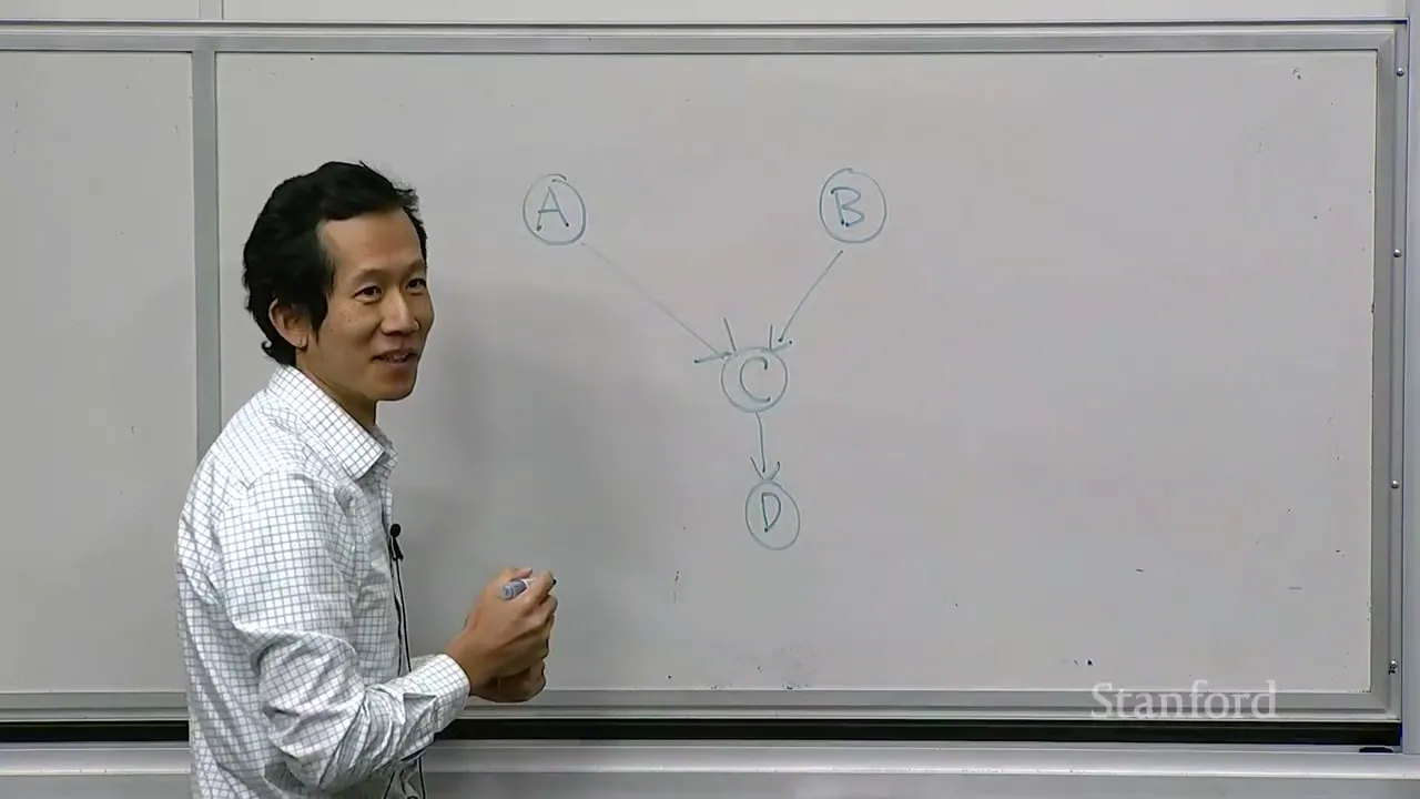
There's an odd little exchange at (40:60) where a student asks why inputs are called leaf nodes if the arrows point away from them. He redraws the graph with arrows pointing down toward the root and admits it's just convention — a node has access to its dependencies, so we draw from the node outward. Not a deep point, but I'm glad someone asked, because the direction convention is exactly the sort of thing that silently confuses people for weeks.
 

Then the chain rule. dC/dA = dC/dB · dB/dA, illustrated with squaring applied twice to get the derivative of a⁴. He mentions he's done this more visually in past versions, in case the code isn't clicking for you.
 

The backward pass is where the conceptual load sits. Each node's gradient is defined as: if I change this node's value by epsilon, how much does the root change? You initialize every gradient to zero, set the root's gradient to one (trivially, nudging the root nudges the root), and then walk backward pushing what he calls "credit or blame" to dependencies.
 

For the square node: the local derivative is 2 times the dependency's value, so 2 × 5 = 10, times the node's own gradient of 1, giving 10 to accumulate into the sum node. For the add node: a change in either input passes straight through, so the node's gradient of 10 gets distributed to both dependencies.
 

The single most valuable moment in the lecture is at (48:54). A student is confused: earlier we said the gradient of x₁ and x₂ means the effect on the root, but now self.grad is 10, the gradient of the sum node — so are we treating the sum node as the root? His answer is the invariant worth memorizing: the root never changes. self is not the root; self is whichever node you're currently visiting. grad always means with respect to the root.
 

Generalized at (50:34): topologically sort the graph, run forward from leaves to root, zero the gradients and set the root to one, then run backward from root to leaves. Backward on a leaf does nothing. Why topological sort instead of a naive traversal? Because it's a graph, not a tree — the same input can feed several nodes, and you need the accounting to come out right.
 

Final picture: every node ends up with a value and a gradient of matching dimensionality. His summary is that this is basically what PyTorch does, just with many more bells and whistles. He also encourages thinking in computation graphs as a way to deepen your understanding of calculus itself, and thanks Isaac Newton for the chain rule.
 

Linear Regression, and the Three Questions That Define Machine Learning

 

At (56:23) the lecture turns from general machinery to the machine learning setting proper, and the tone shifts — this part feels more relaxed, partly because the hard work is done.
 

The task: predict an exam score from hours studied. A predictor is just a function from input to output; his example is 2x + 1. He volunteers that it's a bad predictor, since exam scores don't scale linearly with study hours, but it is a predictor. Then: training data as input-output pairs — 1→4, 2→6, 4→7 — and a learning algorithm that turns training data into a predictor.
 

He frames everything that follows around three questions you have to answer:
 

Which predictors are allowed?​ This is the hypothesis class. Rather than hand-designing one predictor, you define a family and let data pick. For linear predictors, parameters are a weight and a bias, bundled in a small Python data class. Given params (3, 1) and input 1 you get 4; given (2, 0.2) you get 2.2. Infinitely many parameters, therefore infinitely many predictors — but all of them are straight lines. "You can't have squiggly lines."
 

The terminology aside here is useful: in deep learning, "model architecture" is roughly synonymous with hypothesis class, and a model is an architecture plus its parameters, where parameters are just a collection of tensors. He invokes DeepSeek V3 as "a crazy number of very large tensors" that is conceptually no different.
 

How good is a predictor?​ The loss function. The residual is prediction minus target — for params (2, 1) at input 1 against target 4, the residual is −1 — and squaring it gives the squared loss for that example. Average over all examples and you get the training loss: 2 for that predictor, 5.6 for parameters (1, 1). You prefer the first. His mnemonic: "loss is bad."
 

How do we find the best one?​ Optimization, which by this point is mostly review. He computes the gradient of the training loss by averaging the per-example gradients, notes it's two-dimensional because the parameters are, and takes one step: parameters move from (0, 1) to roughly (0.24, 1.09), and the loss drops from 23. Repeat ten times and the loss keeps falling while the gradient norm shrinks, which makes sense — the gradient should be zero at the optimum.
 

The learning rate gets the driving analogy: it controls how fast you go, and there's a trade-off between arriving sooner and crashing. Set it too high and things diverge.
 

Where the Lecture Left Me Unsure

 

A few specific things, since you weren't there to catch them yourself.
 

There's a slip early on that I'd flag if you rewatch. At (22:51) he says the gradient "tells us the direction that decreases the function the most." At (28:43) and again at (1:07:36) he says moving along the gradient increases f the most, and that you have to run the other way. The later statements are the standard ones. If you were taking notes linearly, the first version will quietly corrupt your intuition about gradient descent.
 

The derivation he skips is the one I most wanted. At (1:07:58), having spent twenty minutes arguing that gradients can be computed mechanically and never by hand, he declines to work out the gradient of the linear regression loss — "we already did enough calculus for today" — and just presents the averaged per-example gradients. It's a defensible time call, but it leaves the loop unclosed.
 

Two smaller frictions. The addition node's class is called Sum, and einsum also revolves around summation; combined with einops versus einsum versus the transcription's "Einstein," the naming is doing a lot of double duty in one lecture. And his self.grad notation, while standard for autodiff, genuinely confused a student for two full minutes, which suggests the "gradient is always with respect to the root" invariant deserves to be stated before the code, not after.
 

He's candid where he isn't sure. At (1:10:17), on whether gradient descent would converge to zero if run longer: "I don't actually know." And on convexity — gradient descent is guaranteed to work for convex functions, almost nothing in deep learning is convex, so there's no guarantee of a global minimum, though in practice it works well. That's asserted rather than shown, and SGD and Adam get named but deferred.
 

The thing I'd most want a follow-up on: he says nothing about why squared loss rather than absolute error, and the adversarial examples remark compresses a whole literature into one sentence about pandas and school buses.
 

---

Coming back to the core of it: backpropagation is reverse-mode autodiff over a graph you build out of a handful of primitives, and the whole trick is that each node's gradient means "effect on the root," accumulated backward after a forward pass. If that sentence still feels abstract, the twenty minutes from (36:13) are the part to watch, and the student question at (48:54) is the part that will make it click.
 

Content Disclaimer:

This article is for general reference only and does not constitute professional R&D guidance, production process advice or quality certification. All material performance data has specific test premises; readers should verify parameters against actual equipment and working conditions.