Stanford CS221 ｜Lecture 3： Learning II — Annotated Lecture Notes & Key Takeaways

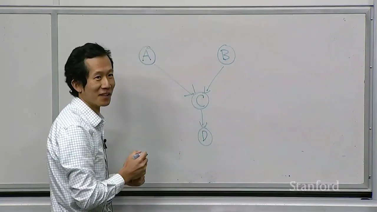
Course Information

Institution: Stanford

Original Course: Stanford CS221 | Autumn 2025 | Lecture 3: Learning II

Instructor Bio: This lecture is delivered by Percy Liang, Associate Professor of Computer Science at Stanford University and core faculty of the Stanford Institute for Human-Centered Artificial Intelligence (HAI). Percy Liang leads the Stanford Natural Language Processing Group and the Center for Research on Foundation Models (CRFM). His research spans the theoretical foundations and practical systems of artificial intelligence, including machine learning, natural language processing, AI alignment, and rigorous model evaluation. He received his PhD in Computer Science from the University of California, Berkeley and his BA in Mathematics from Harvard University. His work has been recognized with the NSF CAREER Award, Google Faculty Research Award, and multiple best paper awards at top-tier AI conferences. He has taught CS 221 at Stanford for over a decade, shaping foundational AI education for thousands of students.

Course Description: This second learning lecture extends foundational supervised learning concepts to classification tasks and more expressive model families. It covers linear classification models including perceptrons and support vector machines, then introduces kernel methods for capturing non-linear patterns in data. The lecture also explores practical learning considerations including feature engineering, L1 and L2 regularization techniques, and model selection methodologies such as cross-validation.

If you missed this one, the short version is that the entire hour turns on a single uncomfortable fact: the thing you actually want to measure in linear classification​ is the thing you cannot optimize. Every other idea in the lecture — the margin, the logistic function, the decision to have a classifier emit probabilities instead of labels — is scaffolding erected to escape that trap. The lecturer walks this path deliberately slowly, and the slowness is the point. He keeps showing you the dead end first, then the detour around it.
 

He opens by replaying the last lecture's setup and asking how much of it survives a change of output type. Regression produced a real number, something like a price or a score, and the hypothesis class was linear functions. Classification produces a discrete choice, one of K labels, where K might be two, five, or a thousand. He hints early that "linear" here is a bit of a lie, since something nonlinear has to happen at the end.
 

From Scoring to Choosing: What Actually Changes

 

Two running examples carry the lecture: image classification (here is a picture, output the object — in this case he thinks it's a cat) and sentiment classification (here is a document, output positive or negative).
 

The input side gets handled unevenly, and he says so. Images are already tensors: width by height by three RGB channels, straightforward. Text is a string, and a string is not a tensor. He waves at that problem and promises to return to it, which he does in the final ten minutes.
 

The output side is where the conventions get pinned down. For binary problems, the label space is −1 and +1 for negative and positive. He acknowledges you'll often see 0 and 1 elsewhere, but this course uses ±1 and that choice matters later, because multiplying by the label turns out to be a neat trick. Multiclass outputs run 0 through K−1 in code and 1 through K in math notation — same idea, different indexing habit.
 

Then he hand-writes a classifier, just to have a concrete object on the board. Take the input vector (1, 2), compute the first component minus the second minus one, which is −2. If that quantity is above zero, predict +1; otherwise predict −1. So (1, 2) comes out negative. A second point, (2, 0), gives a value of 1 and comes out positive.
 

That quantity has a name — the logit — and setting it equal to zero gives you the decision boundary, the line where the classifier is genuinely torn. Plot it in the two-dimensional input space and it slices the plane into a negative side and a positive side. He notes in passing that the tie at exactly zero was broken arbitrarily (zero counted as negative), and you could just as well have used a greater-than-or-equal.
 

The important rhetorical move comes next: none of this is machine learning yet. He wrote that predictor down by hand. Machine learning starts when you have training data — input/output pairs demonstrating the task — and an algorithm that turns that data into a predictor. In two dimensions, "finding a predictor" and "drawing a line that separates the pluses from the minuses" are the same sentence.
 

At (8:03) he lays out the three questions that organize everything: what predictors are allowed (the hypothesis class), how good a given predictor is (the loss function), and how to find the best one (the optimization algorithm). That framework carried the regression lecture, and it carries this one.
 

The Hypothesis Class: Weights, a Bias, and Straight Cuts

 

A linear binary classifier is parameterized by a weight vector and a scalar bias. The logit is the dot product of weights and input plus the bias; the sign of the logit is the prediction. With weights (1, −1) and bias −1, the input (1, 1) produces a logit of −1 and gets classified negative. Keep the weights, change the bias to +1, and the same point lands on the positive side — visually, the boundary slides up past it.
 

So the hypothesis class is every straight cut you can make through the input space, one for each choice of weights and bias. No curves.
 

What follows is the moment I found least satisfying in the first half. He concedes immediately that most real tasks probably aren't linear, calls linearity "a very fragile and special notion," and lists the usual reasons people use linear classifiers anyway: simplicity, few parameters, less overfitting, convexity. Then he reverses and says that in high dimensions — 10,000 of them — linear classifiers are actually very expressive, so "it's not as bad as it looks." Both claims are asserted in about twenty seconds with no example, no geometry, and no hint of why dimensionality changes the picture. I wrote down "ask why" in the margin. He does gesture at neural networks as the escape hatch, so presumably the payoff is deferred, but as a standalone argument it's thin.
 

Three Losses, and the One That Actually Gets Used

 

A loss function takes a predictor and a training set and returns one number: how unhappy should we be. He builds up to the answer by trying two wrong ones first.
 

Squared loss.​ Borrowed from regression, where you measure the residual between prediction and target and square it. Plot it against the residual and you get a bowl with a steep climb on both sides. Applied to classification it technically works — right label gives zero, wrong label gives (2)² = 4 — but the residual concept doesn't really fit a two-valued output. The concrete objection he raises is sharper: with a true label of +1, a logit of 8 gets penalized much harder than a logit of 4, even though 8 means you're correct with enormous confidence. Penalizing confidence is backwards. His verdict is mild — not crazy, just off — and honestly this part would have landed better with a picture. The argument is verbal and quick, and I had to reconstruct the plot myself.
 

Zero-one loss.​ This is the one you actually want. Forget magnitude; just ask whether the prediction has the same sign as the target. Correct gives 0, incorrect gives 1. He computes it twice on the board and then pauses for an aside that I thought was the most useful thirty seconds of the lecture: loss functions are yours to design. Zero-one, logistic, and squared are just names people standardized on. Any function that captures what you care about gives you a valid, custom learning procedure.
 

Then the margin. The logit's sign is the prediction and its magnitude is confidence. Multiply the logit by the true label and you compress correctness into a single number: positive margin means the two signs agree, negative margin means they don't. Zero-one loss becomes "is the margin non-positive." He asks you to sit with that until it's obvious it's the same function, and suggests that margin is to classification what residual is to regression — you plot loss against margin, not against residual.
 

One nice payoff: average the zero-one loss over the training set and you get the error rate. Training loss and misclassification fraction are literally the same number.
 

The Wall: Zero Gradients Everywhere

 

Here's the punchline at (27:15). Differentiate the zero-one loss with respect to the parameters and you get zero almost everywhere, and undefined exactly where the margin is zero. Run gradient descent and the step direction is the zero vector. You don't move. Ever.
 

His explanation is intuitive rather than formal: a gradient is a local instrument. It asks what happens if I nudge the parameters slightly. With zero-one loss, nudging does nothing at all — you have to move a long way to cross the boundary, and there's no gradient pointing you toward doing that. Local methods are simply the wrong tool for a discrete objective.
 

The fix is to change the loss, and he's candid that this is a compromise. You want the loss to capture what you care about; you also want it to be optimizable. Sometimes those pull apart.
 

The way out is conceptual. Instead of a classifier that emits one hard label, have it emit a distribution over labels. The culprit was thresholding — an if-statement is a discontinuous operation, and discontinuity is what erases the gradient. Distributions are continuous objects, so gradient descent has something to grab.
 

The logistic function, and the properties he wants on hand

 

The logistic (sigmoid) function squashes the whole real line into (0, 1). He walks the numbers: zero maps to 0.5, one maps to about 0.73, eight maps to 0.999. Saturation is startlingly fast, which he attributes to the exponential — "whenever you see exponentials, you think like crazy stuff happens."
 

Four properties get flagged for later use. Mirroring: the function at −z equals one minus the function at z, so mirrored logits give complementary probabilities. Derivative: just p(1−p), which peaks at 0.25 when the logit is zero and decays toward zero in both tails — a warning flare about gradients dying, which he says will matter much more for neural networks. Log-odds interpretation: odds are p/(1−p), the log of the odds is the logit, and the logistic function is simply the inverse of that map. And history: the curve is a 19th-century object, first used in statistics as logistic regression in the 1940s, and everything he's about to do is identical to logistic regression.
 

From probability to a loss you can differentiate

 

Declare the logistic of the logit to be the probability of the positive class. By the mirroring identity, the logistic of the negative logit is the probability of the negative class, and the two sum to one. Applied to the margin instead of the raw logit, you get the probability the model assigns to the true label.
 

That's the upgrade he was after. Zero-one loss only told you right or wrong. Now a correct prediction can be 0.5 or 0.97, and you can ask which direction increases it.
 

The principle connecting this to a loss is maximum likelihood: maximize the probability of the training targets. Across multiple examples you'd multiply probabilities, and taking logs turns the product into a sum. Then flip the sign, because optimization frameworks minimize. He frames the choice as temperament: optimists maximize likelihood, pessimists minimize loss, same coin.
 

The resulting logistic loss — negative log probability of the target — has the property he needed. Its curve has nonzero gradient everywhere. He calls it a bit of an overachiever: even at a comfortable margin of 3, it keeps pushing outward, because a bigger margin always means higher probability. That's a feature for optimization and, presumably, a question mark for generalization, though he doesn't raise that here.
 

Why the log? He gives two reasons: training error is conventionally an average over per-example errors, and averaging requires logs; and raw probabilities underflow catastrophically when you multiply many small numbers. The second reason is concrete. The first felt slightly circular to me, since the convention itself is what's in question.
 

Doing the gradient by hand, then watching it work

 

He derives the gradient manually even though, as he says, you could let PyTorch's computation graph handle it — partly because at this scale it's tractable, partly because the algebra exposes structure. The derivative of the loss with respect to the logit works out to the negative logistic of the negative margin; the chain rule then carries it to weights and bias. The gradient has the same shape as the parameters, and the training gradient is just the average over examples.
 

Running it: initialize weights and bias at zero (acceptable for linear models, he notes, but not for neural networks), learning rate of 1, which he admits would be high for anything practical, twenty iterations. The loss curve descends cleanly. The final boundary doesn't hug the points it separates — it pushes away from them, because margin is probability.
 

A student asks where the boundary actually comes from, and the answer is that it's the locus where the logit equals exactly zero. In ten dimensions you'd have eleven numbers instead of three and no way to draw it, but the math and the code are unchanged.
 

K Classes, and What to Do With a String

 

Multiclass is a generalization rather than a new idea. One weight vector per class — a weight matrix — and one bias per class, producing one logit per class.
 

Applying the logistic function to each logit separately fails, because independent probabilities won't sum to one. Probabilities have to be coordinated. The softmax does this by exponentiating every logit and dividing by the sum. He presents it as the lazy route to a distribution: exponentiating makes things non-negative, dividing makes them sum to one, and it happens to also be mathematically pleasant.
 

One property with practical teeth: adding the same constant to every logit leaves the probabilities unchanged. That's the standard numerical-stability trick, since exponentiating large numbers can overflow a machine's finite range. He leaves the proof as an exercise.
 

To turn that distribution into a loss he detours through cross entropy: negative sum over classes of the target probability times the log of the predicted probability. The intuition is exactly what you'd want — get punished for assigning low probability where the target assigns high probability. It's minimized when predicted equals target, and that minimum value is the entropy of the target; subtract the entropy and you get KL divergence, which he points you toward without pursuing.
 

In practice the target is a one-hot vector, and the whole expression collapses to the negative log probability of the true class — the same object as the binary case. He frames it generally so you could also train against a soft target distribution if your ground truth were probabilistic rather than a single label.
 

My one complaint here: having spent real time deriving the binary gradient, he skips the multiclass gradient entirely and tells the class they can do it. Given how deliberately he built everything else, that asymmetry felt abrupt.
 

Turning sentences into tensors

 

The last stretch is dense and fast. Strings need two steps to become tensors. First, tokenization: split on spaces and maintain a vocabulary class that maps each distinct string to an integer index, reusing the index when a word repeats. He's quick to point out that naive space-splitting is a mess — punctuation glues onto words, 3.4 splits into three pieces, German compounds explode — and that modern tokenizers learn the segmentation instead. He names byte-pair encoding and gestures at GPT-2 as the system that pioneered it for language models, flagging the details as out of scope. The transcript is audibly garbled at that point, so I'd treat the attribution cautiously.
 

Second, one-hot encoding: each index becomes a vector with a 1 in that position, and the whole document becomes a sequence-length by vocabulary-size matrix. In practice you never materialize it — indexing rows out of a weight matrix accomplishes the same multiplication far more cheaply.
 

Bag of words just averages those row vectors. The virtue is a fixed-dimensional representation independent of document length, which keeps your parameter count fixed. The cost, which he demonstrates with the classic pair, is that word order vanishes entirely: "dog bites man" and "man bites dog" become identical vectors. He promises transformers as the eventual fix, and notes that the homework uses this representation.
 

The closing summary he gives is a good one to copy into your notes: classification maps inputs to one of K choices; zero-one loss is what you want but can't optimize; so you relax into probabilistic classifiers and optimize the logistic loss instead; multiclass extends it via softmax and cross entropy; and text becomes tensors through tokenization and one-hot encoding.
 

For me, the through-line worth holding onto is that the relaxation from labels to probabilities isn't a modeling preference or a statistical nicety — it's a concession to the optimizer. You accept a loss you don't perfectly want in exchange for one whose gradient is never zero. Everything else in linear classification follows from that trade.
 

Content Disclaimer:

This article is for general reference only and does not constitute professional R&D guidance, production process advice or quality certification. All material performance data has specific test premises; readers should verify parameters against actual equipment and working conditions.