Stanford CS221 | Autumn 2025 | Lecture 10: Games I — Annotated Lecture Notes & Key Takeaways

Course Information

Institution: Stanford

Original Course: Stanford CS221 | Autumn 2025 | Lecture 10: Games I

Instructor Bio: This lecture is delivered by Percy Liang, Associate Professor of Computer Science at Stanford University and core faculty of the Stanford Institute for Human-Centered Artificial Intelligence (HAI). Percy Liang leads the Stanford Natural Language Processing Group and the Center for Research on Foundation Models (CRFM). His research spans the theoretical foundations and practical systems of artificial intelligence, including machine learning, natural language processing, AI alignment, and rigorous model evaluation. He received his PhD in Computer Science from the University of California, Berkeley and his BA in Mathematics from Harvard University. His work has been recognized with the NSF CAREER Award, Google Faculty Research Award, and multiple best paper awards at top-tier AI conferences. He has taught CS 221 at Stanford for over a decade, shaping foundational AI education for thousands of students.

Course Description: This lecture opens the game theory module, introducing multi-agent strategic interaction as a core AI problem domain. It covers normal-form games, the Nash equilibrium concept, dominant strategies, and the minimax theorem for zero-sum games. The lecture also explores algorithms for computing equilibria in two-player zero-sum games, including minimax search with alpha-beta pruning for adversarial search problems such as board game AI.

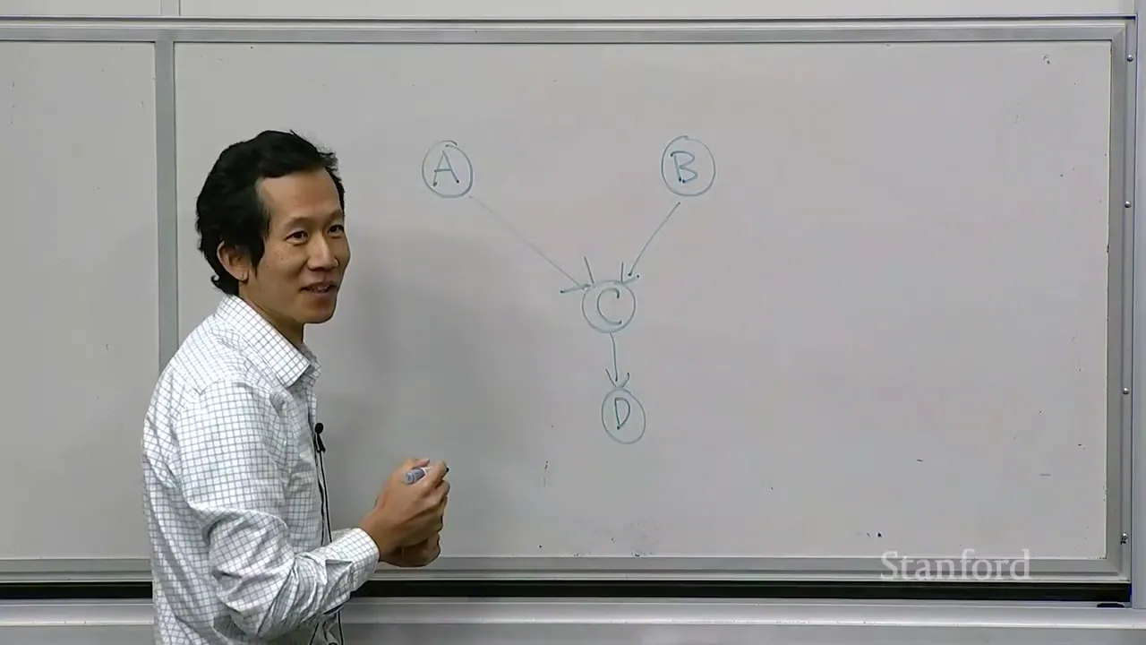
The lecture opens with a poll, and the poll is the whole thesis in miniature. There are three bins, A, B and C. You pick one, the lecturer then picks a number out of it, and your payoff is that number. Most of the room went with C. A handful went with A. He says he is surprised more people didn't pick B — "you guys don't think I'm as adversarial as I might be" (0:34).
 

What makes the question interesting is that it is deliberately underspecified. Bin A might contain a 50 or it might contain a −50, and which one you get depends entirely on what he decides to do. Your answer should be a function of his behaviour, and you don't know his behaviour. That is the entire difficulty of games, compressed into thirty seconds of classroom theatre.
 

Why Games Aren't Just MDPs with a Mean Environment

 

The clean statement of the contrast comes at about the two-minute mark. In a Markov decision process the agent maximises utility and the environment is stochastic; if the transition model is unknown you do reinforcement learning until it becomes known, implicitly or explicitly. In a game the agent is still maximising utility, but the randomness has been replaced by another decision-maker whose policy is unknown.
 

That sounds like a small edit and it is not. An environment that rolls dice doesn't care what you do. An opponent reads you, and the policy that is brilliant against a sloppy opponent can be terrible against a careful one. Everything after this point — every recurrence, every guarantee, every hedge — is the class working out what to do when the thing you're optimising against is also optimising.
 

The roadmap he gives (2:34) is worth holding onto, because the lecture really does follow it: first modelling (what is a game?), then how you actually play one and what "the value of a game" could mean, then a stack of recurrences for optimal values and policies, then two ways to make the whole thing faster — one exact, one approximate.
 

The Game Tree, and a Second Example That Actually Tests You

 

The central object is the game tree. Root is the start state, edges are actions, and any root-to-leaf path is one rollout — one complete play of the game. Some nodes are yours, some are the opponent's.
 

The running example, drawn on the board, is the bin game. If you pick A, the opponent chooses between −50 and 50. Pick B and the choice is between 1 and 3. Pick C and it's between −5 and 15. Keep those six numbers in your head; he reuses the same tree for four different recurrences later, and watching the numbers get recombined is where the lecture earns its keep.
 

The class restricts itself to two-player zero-sum games (4:23). Zero-sum means the two utilities always add to zero, so anything good for you is exactly as bad for the opponent.
 

Formally, a game gives you a start state, an end-of-game test, a successor function mapping an action to the next state, a utility attached to terminal states, and — this is the genuinely new piece relative to search and MDPs — a function telling you whose turn it is at any given state. The state itself carries the turn. That sounds like bookkeeping, and it is, but it's load-bearing: because turn order lives in the state, you can later express things like "this player gets two moves in a row" without changing the framework at all.
 

Two properties make games harder than the models that came before. First, all the payoff sits at the terminal node. He connects this to the sparse reward problem in reinforcement learning — you can appear to be cruising and then have it all fall apart on the last move. Second, control alternates between two agents rather than between an agent and a chance node.
 

The second example is the halving game (9:18). You start with a number, say 11. On your turn you either subtract one or halve and round down. Whoever is handed zero wins. He shows the tree branching off 11 into 10 and 5, and declines to tell you the right answer, noting that you'd need to run the minimax recurrence in your head to see it. It's a better example than the bins because you can't eyeball it.
 

One small aside that cleared something up for me: there is no discounting in this lecture. When the entire utility is one terminal number, there is nothing to discount.
 

Four Recurrences, All on the Same Little Tree

 

This is the bulk of the lecture, and the structure is a ladder. Each rung changes one line of the previous recurrence.
 

Game evaluation

 

Fix a policy for both players and the value of the game is the expected utility over all rollouts. The recurrence is the obvious one: at a terminal state return the utility; otherwise look at whose turn it is and take a probability-weighted average over successors, using that player's policy for the weights.
 

It's exact, and it's exponential. He gives the throwaway figure of two actions per node over a hundred steps, which is 2^100 — not a computation you get to finish.
 

The alternative is simulation, and he uses it to make a nice point about sampling error. Running the agent policy "always choose A" against a coin-flipping opponent twenty times gave an average of 15. Run it a million times and it converges to 0, which is what you'd expect when the two leaves are −50 and 50. The 15 was noise.
 

Under that same random opponent, the three bins evaluate to 0, 2 and 5 respectively. Game evaluation, he notes, is exactly policy evaluation in MDPs.
 

Expected max

 

Now let the agent optimise while holding the opponent's policy fixed (20:44). One line changes: at agent nodes, instead of averaging over the agent's policy, you take a max over successors. Opponent nodes still average, because the opponent's policy is given and known.
 

The practical consequence is that you lose the ability to estimate by sampling. Averages you can sample; maxima you can't, because the max of sampled averages is biased in a way that averages of samples aren't.
 

On the bin game, expected max picks C and scores 5. He makes the psychological point explicitly: if you chose C at the start, you were probably doing expected max in your head, assuming he'd flip a coin and hoping the −5 wouldn't come up. He likens this to value iteration.
 

Minimax

 

Here the opponent's policy stops being given (26:19). The principle is to assume the worst: the opponent plays as well as possible and minimises your utility. The recurrence is now the simplest one on the board — max at your nodes, min at the opponent's.
 

Run it on the bins and the character of the game inverts. Bin A's min over {−50, 50} is −50. Bin B's min over {1, 3} is 1. Bin C's min over {−5, 15} is −5. The root takes the max of those, which is 1, and the optimal move is B. The people who answered B were, he says, running minimax in their head; of the people who answered A, he has no explanation to offer.
 

Turning that into a policy is just: at every state you actually reach, recompute and play the argmax action. In the halving game, the resulting agent beat a random opponent in all ten simulated games. He also shows the minimax values for the first eleven states, and explains what they mean. A value of +1 means the win is guaranteed no matter what the opponent does. A value of −1 means the opponent wins if the opponent plays optimally — which is not the same as saying you've lost, because a weaker opponent can still hand it back.
 

There's a nice aside on the word "solved." A game is strongly solved when you know the minimax value of every position — tic-tac-toe, nim, Connect Four. Weakly solved means you know it only from the opening position. Chess and Go are neither, and he's firm about this: engines beat humans, but that doesn't mean we know the game-theoretic value of the opening or the optimal policy. We just have policies better than ours.
 

The reason minimax is where games stop being MDPs is the closing line of this stretch: MDPs only ever max and average. They never min.
 

Expectiminimax, and where the framework stops

 

As a kind of dessert, he adds a coin flip. You choose a bin, then a fair coin decides whether he draws from your bin or shifts one bin to the left, wrapping around. You model this by inventing a "coin" pseudo-player with a fixed stochastic policy, and the recurrence grows a third case: max for you, min for him, average for the coin.
 

From there he gestures at what else fits. Multiple players (the Pac-Man assignment has several ghosts), extra turns, choosing who moves next — all of it is expressible, because turn order is just a field in the state.
 

What doesn't fit matters as much. Imperfect information — poker, most card games — breaks the model, because everything in these trees has to pass through a single shared state and there's no way to give two players different views of it. Non-zero-sum and cooperative settings like the prisoner's dilemma are out of scope by assumption. So are simultaneous-move games; turn-based rock-paper-scissors would be, as he puts it, pretty boring.
 

"Optimal" Is Always Optimal Against Somebody

 

This is the densest stretch of the lecture, around the 41-minute mark, and it's the part I'd most want to rewatch.
 

The warning is simple and easy to forget: never say "the optimal policy" without asking, optimal with respect to what. He lines up four policies — the minimax agent, π_max; the minimax opponent, π_min; an expected-max agent tuned against some arbitrary fixed opponent; and that arbitrary opponent itself. Then he plays them against each other in a two-by-two table and asks what relationships the numbers must have.
 

Three properties do the work. π_max is the best response to π_min, so swapping in any other agent can only lower the value. π_min is the best response to π_max, so swapping in any other opponent can only raise it — which is another way of saying the minimax value is a floor. And the expected-max agent is the best response to the specific opponent it was tuned against, so π_max can only do worse against that opponent.
 

Chain them together on the bin game and you get a strict ordering: expected-max against the worst-case opponent scores −5; the minimax value is 1; minimax against the random opponent scores 2; expected-max against the random opponent scores 5. The fact that all four numbers fall into line isn't a coincidence, it's the three properties.
 

The payoff is a real guarantee. If minimax returns 1 in a win/loss game, you win no matter what the opponent does, and now you can see formally why: deviate downward and the value can only rise.
 

He also states a preference that I found more interesting than the theorem. You can read minimax two ways — as a best response to a perfect adversary, or as a lower bound against an opponent you know nothing about. He says he prefers the second reading, because you're rarely actually facing the worst possible opponent.
 

My quibble is that the second reading quietly hides a cost, and his own table shows how big it is. Committing to minimax against the coin-flipping opponent scores 2; exploiting that opponent scores 5. He does say you can do better than minimax when you know your opponent, but he moves on quickly. Worst-case reasoning is a floor, not a strategy, and the gap between the floor and what's available can be wide. That's worth sitting with before you make worst-case your default.
 

Cutting the Tree Down: Alpha-Beta and Evaluation Functions

 

Alpha-beta pruning

 

The exact speedup (52:13). The intuition is a comparison he puts to the room: option A will pay somewhere between 3 and 5, option B somewhere between 5 and 100. You don't need to resolve either number to know you want B. This is branch and bound.
 

Mechanically, you maintain bounds as you search. Max nodes accumulate a lower bound on their value (alpha); min nodes accumulate an upper bound (beta). The minimax value of the whole tree has to come from some leaf, and the path that the two policies would take to that leaf has to remain inside every ancestor's bounds. So the moment a node's interval stops overlapping the intervals above it, the entire subtree below is dead and you walk away.
 

The board example goes roughly like this: you descend, find a 9, then a 7, which pins that min node at 7 and propagates a lower bound of 7 to the root. In the next subtree the first leaf is a 6, which caps that min node at 6 — already below 7 — so everything under it gets cut without being looked at. Further along, a child that yields 8 still overlaps the [7, ∞) window at the root, so you're forced to keep exploring, and the final leaf settles the value at 7.
 

Ordering is what makes or breaks it. Search children in the order (3, 5) then (2, 10) and the 10 gets pruned for free; search them as (2, 10) then (3, 5) and you prune nothing. The practical rule is to order max-node children by decreasing guessed value and min-node children by increasing guessed value, using a heuristic to make the guesses. He draws the parallel to A* explicitly: a good heuristic makes you fast, a bad one makes you slow, and neither makes you wrong. It's still exponential in the worst case — "it's not like we've solved P = NP."
 

Two honest notes here. A student asked whether alpha-beta carries over to expected max, and the answer was no in general, because an expectation has to account for every branch; the lecturer allowed that bounded utilities might permit some pruning and then admitted he'd have to think about it. So the recurrence that mixes chance with an adversary is the one with no clean exact speedup. I also found the board work genuinely hard to follow from a recording — he's drawing nodes live and reading numbers aloud, the leaf values blur together, and I had to replay the interval logic twice before the pruning step felt obvious. A printed tree would have fixed that in one slide.
 

Evaluation functions and depth-limited search

 

The approximate route (67:38). Instead of searching to a terminal state, you just score the position you're in. For chess he sketches the classic weighted sum: material (queen worth nine, rook worth five), mobility, king safety, control of the centre. Each term is a feature you believe correlates with winning.
 

Used on its own, this is a bad player. It's greedy — it hoards material and misses the point.
 

Used inside search, it's the standard trick. Depth-limited search runs the minimax recurrence but stops at a fixed depth and returns the evaluation function instead — his phrase for it was a "vibe check" (69:09). One detail worth catching: depth only decrements on the opponent's move, so a single unit of depth corresponds to a full pair of turns.
 

There are no optimality guarantees. What you do get is a dial. Search deep and a mediocre evaluation function matters less, because the search compensates. Search shallow and the evaluation function had better be sharp. He closes by pointing at the connection to reinforcement learning: an evaluation function looks a lot like a value function or a Q-value, which means it can be learned rather than hand-designed — and that's next lecture's topic, TD learning.
 

Where That Leaves You

 

The through-line of the hour is a ladder of assumptions. Average over both players and you're doing MDPs. Max over yourself and average over a known opponent and you're doing expected max. Max over yourself and min over an unknown opponent and you're finally doing something with no analogue in anything that came before. Every rung is a different claim about how much you trust your model of the other player, which is why "optimal" never means anything on its own here.
 

If you take one thing away, take the ordering of those four numbers — −5, 1, 2, 5. It encodes what each policy is promising you and what it's assuming, and it's the fastest way I know to see why minimax is a floor rather than a target.
 

Content Disclaimer:

This article is for general reference only and does not constitute professional R&D guidance, production process advice or quality certification. All material performance data has specific test premises; readers should verify parameters against actual equipment and working conditions.