Stanford CS221 ｜ Autumn 2025 ｜ Lecture 13： Bayesian Networks and Gibbs Sampling.en_Transcript — Annotated Lecture Notes & Key Takeaways

Course Information

Institution: Stanford

Original Course: Stanford CS221 | Autumn 2025 | Lecture 13: Bayesian Networks and Gibbs Sampling

Instructor Bio: This lecture is delivered by Percy Liang, Associate Professor of Computer Science at Stanford University and core faculty of the Stanford Institute for Human-Centered Artificial Intelligence (HAI). Percy Liang leads the Stanford Natural Language Processing Group and the Center for Research on Foundation Models (CRFM). His research spans the theoretical foundations and practical systems of artificial intelligence, including machine learning, natural language processing, AI alignment, and rigorous model evaluation. He received his PhD in Computer Science from the University of California, Berkeley and his BA in Mathematics from Harvard University. His work has been recognized with the NSF CAREER Award, Google Faculty Research Award, and multiple best paper awards at top-tier AI conferences. He has taught CS 221 at Stanford for over a decade, shaping foundational AI education for thousands of students.

Course Description: This lecture covers approximate inference methods for Bayesian networks when exact inference is computationally intractable for large or dense models. It focuses on Markov Chain Monte Carlo (MCMC) methods, with detailed coverage of Gibbs sampling and the Metropolis-Hastings algorithm. The lecture explains convergence properties of sampling methods, practical considerations for effective MCMC inference, and applications to large-scale probabilistic reasoning problems.

Lecture 13 is one of those sessions that opens like a review and then quietly gets hard. The billing says Gibbs sampling and conditional independence. What actually arrives is a fairly complete argument for why approximate inference is unavoidable, one concrete trick for making it cheaper, and about forty seconds of the conditional independence topic before the recording I have runs out. I'll flag that gap at the end, because I think it matters for how you study this material.
 

The spine of the lecture is a comparison between two sampling algorithms — the one from last time (rejection sampling) and today's (Gibbs). The lecturer is unusually candid about the fact that both of them fail, and that they fail for opposite reasons. If you take one thing away, it's probably the diagnostic question at the end: is your problem hard because the evidence is rare, or because the variables are welded together?
 

The Four-Step Setup: A Bayesian Network Is a Database You Query with Probabilities

 

The review portion restates the construction as a four-step procedure. You decide what the variables are, you draw a directed graph over them, you attach a numeric conditional table to each node given its parents, and you multiply those tables together to get a joint distribution. The lecturer's image for this is memorable: the graph is the bones, the tables are the meat you hang on them.
 

The example is the usual burglary / earthquake / alarm trio. Burglary and earthquake each get a prior of 0.05 and are treated as independent; the alarm depends on both. What I found genuinely clarifying was the alarm's table. Because the alarm is a deterministic function — it fires when a burglary or an earthquake happens — the table is just a stack of zeros and ones, which the lecturer openly calls a comically roundabout way of writing down a logical OR. That's a useful thing to see early, because it kills the assumption that every entry in a conditional table has to be a "learned" probability. Sometimes a table is just encoding a rule.
 

He also shows the tensor view, multiplying the local tables together with einsum notation and tracking which index lines up with which variable. For three boolean variables you get eight numbers, and he's explicit that you could have written those eight numbers down directly — the point of going through the structured route is interpretability rather than compactness. Eight arbitrary floats tell you nothing about the world; eight floats assembled from "burglaries are rare" plus "alarms fire on either cause" tell you a story.
 

The framing I'd write on a flashcard: the joint distribution is a database, and probabilistic inference is the query language. SQL is to a table as conditioning and marginalizing are to this one.
 

The worked query is P(burglary | alarm). The mechanics are worth internalizing because the rest of the lecture is about avoiding them. You take the joint tensor, slice it down to the rows where the alarm fired, collapse away the earthquake variable by summing over its two values, and then divide through by the total mass of the surviving rows. The answer is 0.51. He mentions this presentation differs from last lecture's and that he thinks it's more intuitive; I'd agree, the slice-then-collapse ordering maps cleanly onto what you'd do in code.
 

The Exponential Wall, and What Rejection Sampling Does About It

 

Then the wall. A hundred binary variables means 2¹⁰⁰ assignments (10:03), and nobody is writing that down. So the honest goal becomes approximation, delivered with a shrug: you approximate and hope for the best.
 

The bridge to sampling is the idea of a probabilistic program — a program whose job is to return one sample from the joint, which means the program is the distribution in any practical sense. The alarm network becomes four lines: flip a coin for burglary, flip one for earthquake, set the alarm to their OR, return the assignment. Run it twice, get two independent draws.
 

Rejection sampling then wraps that program. You declare a query (pull out the burglary value) and an evidence test (check whether the alarm fired). Draw a sample, test it, and only if it passes do you bump a counter for the query value. Normalize the counters at the end.
 

There's a nice student exchange here about why the running total isn't just the number of samples — because most samples get thrown away. And the accuracy number is sobering: 300 samples put P(burglary | alarm) at about 0.44 against the true 0.51. A million samples converges, but 300 is only in the neighborhood.
 

Rejection sampling's two structural wastes

 

The diagnosis of why it's slow has two parts, and I want to separate them because only one of them gets fixed later.
 

First, every draw starts from scratch. Nothing learned from the previous sample carries forward. Second — and this is the killer — the program generates a whole assignment without ever consulting the evidence, then prays the evidence happened. If the thing you're conditioning on has probability around 10⁻³⁰, you will be rejecting until the heat death of the universe.
 

I appreciated that he doesn't trash the algorithm. He calls it the fastest path from "I have a Bayesian network" to "I have an inference algorithm that provably works in the limit." Simplicity counts for something, especially on a problem set.
 

Gibbs Sampling: Editing One Variable at a Time

 

Gibbs flips both wastes. Instead of generating fresh, you keep a single assignment alive and gradually mutate it. Instead of ignoring the evidence, you initialize to something that already satisfies it, so there is no rejection step at all (15:44).
 

The cost is that consecutive samples are no longer independent. Ten independent rejection samples beat ten Gibbs samples, because the Gibbs ones resemble each other. This is where the MCMC label comes in — a Markov chain Monte Carlo method, a sequence of draws each depending on the last (17:38).
 

The running example is the children's game telephone, modeled as a chain: a random bit at A, then 0.8 chance of preserving the bit at each hop into B and into C. The question is what the last person's message tells you about the first, concretely P(A = 1 | C = 1). Rejection sampling with 100 samples estimates 0.65.
 

The algorithm itself: initialize to an assignment consistent with the evidence, then sweep through the variables in round-robin order. For each one, compute its conditional distribution given the current values of every other variable by evaluating the joint at each of that variable's possible values, normalizing those few numbers, and drawing from the result. Record the query variable's value after each update. Evidence variables are simply never resampled — C stays pinned at 1 because that's what we're conditioning on.
 

Walking through one resampling step

 

The arithmetic he does on the board is the part I'd replay. Starting from (A=1, B=0, C=1), consider flipping B. Both B=0 and B=1 get scored by the joint: the 1-0-1 path requires two errors and scores about 0.02, while 1-1-1 requires none and scores about 0.32. Normalized, that's roughly a 94% chance of dragging B up to one. The intuition is that hearing a 1 at the far end makes a double-flip story much less attractive than a clean transmission. But it's still probabilistic — about 6% of the time the sample stays put.
 

A student asks why only one variable moves at a time, and the answer is the real design insight: freezing everything else means you can brute-force the full domain of a single variable and stay cheap. One variable is exhaustive; all of them at once is 2¹⁰⁰ again.
 

The cost formula he gives is iterations × variables × domain size × variables, that last factor because scoring even one modified assignment technically walks every local table. Gibbs run on the telephone network lands at 0.68 against rejection's 0.65 — same ballpark, different algorithm, and he's careful not to claim either is right.
 

The Markov Blanket Trick: Cancel the Factors That Don't Touch You

 

That last cost factor is what the middle of the lecture attacks (43:33). Look at the expression for resampling A given B and C, and the term for C given B appears in both the numerator and the denominator. Whether it evaluates to 0.1 or 0.2 is irrelevant — it cancels. So you can drop it, along with any other factor that doesn't involve the variable being resampled.
 

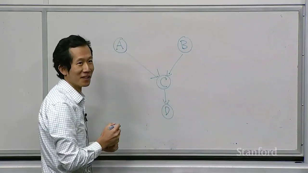
What survives is the Markov blanket. The first definition offered is parents plus children. Then someone asks about co-parents, and the answer is yes, you need those too — if your child also has another parent, that parent's value changes how your value gets translated, and the parents of a node act as a unit. On the A→B→C chain this is easy: A's blanket is just B, B's blanket is A and C, C's is B.
 

One point that was hard to follow here is that the definition gets stated cleanly and then quietly amended in response to a question, so if you were copying notes you may have written down "parents and children" and stopped. The correct version, as he confirms with the example, includes your children's other parents.
 

The payoff is that scoring a candidate value now scales with the size of the blanket instead of the size of the whole network, and the results are identical to the full-joint version up to floating point. His own framing of the win is modest and I like it: it doesn't fix anything fundamental about Gibbs, it's just — why not do it? If blankets are large, you save nothing, but you lose nothing either.
 

Where Each Sampler Breaks, and the Cliffhanger Nobody Resolved

 

The last stretch is the most useful part of the lecture and also the most uncomfortable, because the numbers misbehave on camera.
 

Running Gibbs on the alarm network — the same network where the exact answer is 0.51 — gives 0.6 on one run and 0.33 on another with 200 iterations. That's not a rounding wobble. The lecturer's response is honest: these are approximate algorithms and your mileage varies, so pay attention to the conditions under which a given one works (50:25).
 

Then the two failure modes, built as mirror images.
 

Rejection sampling dies on rare evidence. A two-variable network where B=1 is roughly a one-in-ten-thousand event makes rejection sampling keep one sample in ten thousand, while the actual answer — two-thirds — is sitting right there in two rows of the joint. Gibbs nails this instantly, because it starts inside the rare event and never leaves.
 

Gibbs dies on correlation. Take A as a fair coin and B exactly equal to A, with no evidence at all. Rejection sampling has no trouble, since there's nothing to reject. Gibbs starts at (0,0), tries to move A, finds that A=1 given B=0 has zero probability, tries B, same story — and sits there forever, confidently reporting that A is always zero when the truth is 50/50. The analogy is a three-legged race: you're tied to your partner and neither of you can move until the other does (56:46). He notes that loosening the link to 0.9999 doesn't rescue you, it just makes escape improbable rather than impossible.
 

The bleak summary is hard to argue with: rejection sampling struggles with rare events, Gibbs struggles with tightly coupled variables, and most real problems have both.
 

He gestures at the escape hatches without opening them — Metropolis-Hastings as the more general MCMC scheme with a proposal distribution, and mixing times as the theory for how long these chains take to wander (57:59). Gibbs stays popular because it's simple and effective, with the caveat that it can also be quite slow.
 

Two things I'd have liked and didn't get. The 0.6-versus-0.33 spread is attributed to randomness, but with correlated samples I wanted a discussion of burn-in and whether every sweep should really be counted as a fresh observation — that section would benefit from even one sentence on it. And the conditional independence topic (58:44) is only introduced: the observation that a Bayesian network is simultaneously a probabilistic object and a combinatorial one, and that graph structure should tell you something about independence. That's exactly the bridge from Gibbs back to exact inference, and my recording ends right as he says it.
 

Practically, the takeaway I'd act on is a triage rule: if your evidence is vanishingly rare, don't even reach for rejection sampling; if your variables are near-deterministically linked, Gibbs will lie to you with total confidence. Diagnosing which one you have is worth more than tuning iteration counts.
 

Content Disclaimer:

This article is for general reference only and does not constitute professional R&D guidance, production process advice or quality certification. All material performance data has specific test premises; readers should verify parameters against actual equipment and working conditions.