Stanford CS221 | Autumn 2025 | Lecture 12: Bayesian Networks I — Annotated Lecture Notes & Key Takeaways

Course Information

Institution: Stanford

Original Course: Stanford CS221 | Autumn 2025 | Lecture 12: Bayesian Networks I

Instructor Bio: This lecture is delivered by Percy Liang, Associate Professor of Computer Science at Stanford University and core faculty of the Stanford Institute for Human-Centered Artificial Intelligence (HAI). Percy Liang leads the Stanford Natural Language Processing Group and the Center for Research on Foundation Models (CRFM). His research spans the theoretical foundations and practical systems of artificial intelligence, including machine learning, natural language processing, AI alignment, and rigorous model evaluation. He received his PhD in Computer Science from the University of California, Berkeley and his BA in Mathematics from Harvard University. His work has been recognized with the NSF CAREER Award, Google Faculty Research Award, and multiple best paper awards at top-tier AI conferences. He has taught CS 221 at Stanford for over a decade, shaping foundational AI education for thousands of students.

Course Description: This lecture introduces Bayesian networks as the primary graphical framework for probabilistic reasoning under uncertainty. It covers the graphical representation of joint probability distributions, conditional independence semantics, and the chain rule for efficient factorization. The lecture also explains exact inference algorithms including variable elimination, and analyzes the computational complexity of probabilistic inference across different network structures.

The lecture I sat through is the point in Stanford's CS221 where the course stops asking "what action should I take?" and starts asking "what does the world look like?" That shift is what Bayesian networks are for, and the instructor spends most of the hour building them up from scratch: a short recap of where the class has been, a re-teaching of basic probability using tensor notation, and then two worked examples — a burglar alarm and a fake medical diagnosis — that both land on the same counterintuitive phenomenon he calls explaining away. Fair warning about the recording I used: it runs to roughly the sixty-minute mark and cuts off mid-sentence, right as he starts writing down the general form of a probabilistic inference query. So this is part one of a story that continues in the next lecture.
 

Why the Course Pivots Here: Cheap Reflexes Versus an Actual Model

 

He opens by redrawing the map of the term. The four ingredients of intelligence from the first week were perceiving, reasoning, acting, and learning, and the first stretch of the course covered the perceive-and-act loop: train a predictor, linear or a deep net, feed it what the sensors give you, get a prediction or an action out.
 

Then came the reasoning half, and he walks through it as a ladder of increasingly hostile worlds (0:54). Search problems, where an action has one deterministic consequence and you can hunt for a minimum-cost path. Markov decision processes, where the outcome is stochastic but the distribution over outcomes is known, which makes value iteration possible. Games, where the rules are known but there's an adversary with an unknown strategy, so you end up being conservative and running minimax.
 

Across all three, he says, the class looked at two postures. Model-free methods learn just enough to choose actions and estimate utility — classification, regression, SARSA, Q-learning, TD learning. Model-based methods insist on understanding how the world actually works, on knowing what follows from what, so you can plan.
 

The argument he makes for caring about the second posture is concrete rather than philosophical. If you own a model, you can change the reward function on the fly, keep the transition dynamics fixed, and recompute an optimal policy. A Q-value can't do that, because it has already compressed rewards and transitions into a single number — it has no way to tell you whether an action looks attractive because good outcomes are likely or because good outcomes are valuable.
 

He's honest about the trade-off, and this is the part I'd underline if you're deciding how much to care. Model-free is direct and cheap, which is why, in his words, plenty of practical work just reaches for it. Model-based is harder, because knowing which action to take is a strictly easier problem than understanding the world. He's buying the harder problem anyway, and then he poses the question that drives the rest of the hour: if we're modeling the world, how on earth do we represent its state?
 

Probability, Re-taught as Tensor Gymnastics

 

The answer starts with a probability refresher that he openly flags as "unorthodox." The unorthodox part is that he does everything in Einstein summation notation — he keeps calling it "inops," which is the transcription mangling einsum — because every probability table is really just a tensor, and all the laws of probability turn out to be einsum operations.
 

He sets up two binary variables: S for whether the sun is out, R for whether it's raining. Four assignments, four probabilities: no sun no rain is 0.2, no sun with rain is 0.08, sun without rain is 0.7, sun and rain together is 0.02. The last one is small because it's unusual to get both at once, and the sun-without-rain entry is large because, as he puts it, we're in California. The 0.2 case gets a shrug: no sun and no rain, so probably night.
 

At around 7:36 he switches to code and introduces a class that wraps a NumPy array, with rows indexed by one variable and columns by the other. He also shows the same table "rolled out" into a flat list of assignment–probability pairs, and the reason is pure practicality: once you have four variables you can't draw a four-dimensional tensor on a blackboard. I appreciated that he bothered to justify the notation change instead of just switching representations.
 

Marginalization: Throwing Away Distinctions You Don't Care About

 

The first operation is marginalization, and the mental image he offers is collapsing rows. To get the probability that the sun is out, you take the assignments that differ only in R and add them together: 0.2 plus 0.08 gives 0.28 for S = 0. Pictorially it's the first two rows merging, then the second two. Marginalize several variables at once and you collapse many more rows, and the output table is smaller than the input.
 

This is where the tensor notation earns its keep. The formula — probability of S equals the sum over R of the joint — becomes a one-liner, because the rule is simply that any index appearing on the left but not on the right gets summed out. There's a small wart he acknowledges: the probability table object has an accessor for the underlying tensor, so expressions pick up a stray .p. He calls it a notational nuisance and tells people not to worry about it.
 

Conditioning: Select, Then Renormalize

 

Conditioning is the other operation, and it happens in three moves. You condition on a partial assignment — say R = 1, it's raining — which means selecting only the rows consistent with that evidence and ignoring the rest. Then you compute the probability of the evidence itself by adding up whatever survived selection; in this example, 0.08 plus 0.02 is 0.1. Then you divide.
 

The result is 0.8 and 0.2. He has a nice way of phrasing why the division matters: the surviving probabilities are tiny, because rain is rare by itself, and conditioning asks you to suppose the rare thing already happened. Dividing by the probability of the evidence blows the surviving numbers back up so they sum to one. Selecting, then renormalizing.
 

A student asks whether any of this carries over to continuous variables, and the answer is a deferral: everything in the course uses discrete variables, continuous cases need integrals instead of sums, and conditioning on continuous values gets dicey because you can end up conditioning on an event of probability zero. He says you have to be careful and moves on. If you were hoping for the continuous story, it isn't here.
 

His recap at 19:38 is worth memorizing. The joint distribution is the source of truth — for every possible state of the world, how likely is that state. Marginalization means ignoring differences along some variables. Conditioning means you observed something, you select by it, you price the evidence, and you divide.
 

Probabilistic Inference, Framed as Querying a Database

 

Inference gets introduced with four variables instead of two: sunshine, rain, traffic, and whether it's autumn. The joint distribution now has sixteen entries, and the question he poses is what's the probability of rain given that there's traffic and it's autumn.
 

The analogy he wants you to hold onto is that the joint distribution is a SQL database and probabilistic inference is running queries against it. You have the table of facts, you ask a question. He mentions in passing that there's a much more formal relationship between the two than the analogy suggests, and then explicitly declines to get into it.
 

The shape of every query is the same, and this is the bit that would save you on a homework set. There's evidence — a subset of variables pinned to particular values. There's a query variable you want a distribution over. And any variable in neither set is implicitly marginalized away. In the four-variable example, sunshine appears nowhere in the question, so it gets collapsed silently.
 

Building a Network: Earthquakes, Burglaries, and a Very Rude Alarm

 

At 23:45 he starts the first real Bayesian network, and he's upfront that nothing so far has been Bayesian: networks get built on top of probability, and their whole purpose is making joint distributions easier to specify.
 

The scenario (24:25): earthquakes and burglaries are independent, each with probability 0.05, which he concedes is high. You have an alarm that goes off if there's either one. You're away on a trip, your phone shows the alarm is sounding, but the alarm doesn't tell you why. Then you check the news and see there was an earthquake near your house. Question: what does that do to the probability of a burglary?
 

He runs a three-way poll — does it go down, go up, or stay the same — and then names the tension out loud. Intuition says down. But the two causes are independent, and what do burglaries and earthquakes have to do with each other? He calls it a paradox and asks people to hold on.
 

The resolution comes from building the thing properly, and the build has four steps.
 

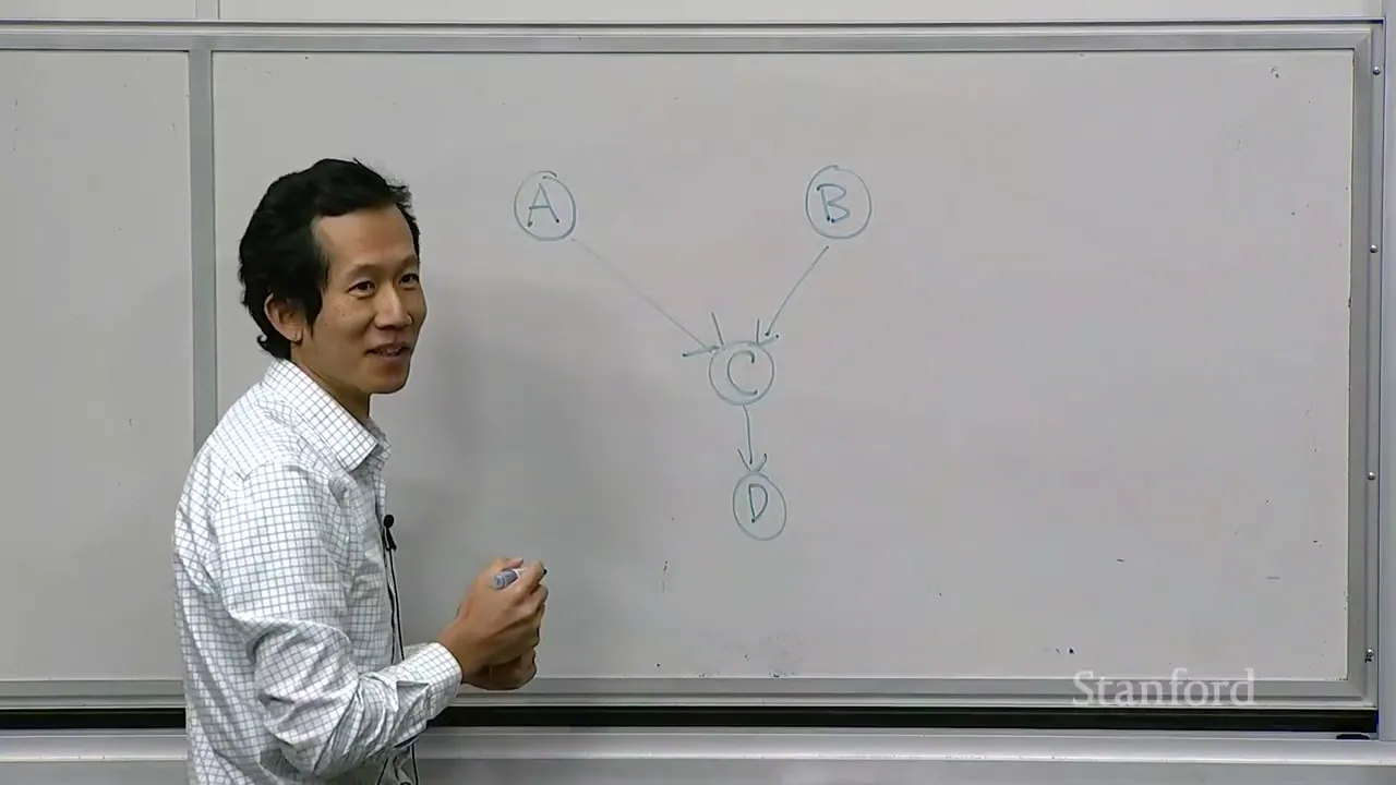
You name the variables: B for burglary, E for earthquake, A for alarm. You draw directed edges, which he says indicate direct influence, and here he slows down to issue a caveat — the natural reading is causation, but causality is a tricky topic and Bayesian networks don't automatically imply it. You're welcome to think "causes" for intuition, he says, just know it isn't fully formal. Then I'd flag this as the slipperiest moment in the whole hour: he spends thirty seconds warning you off the causal reading and then immediately invites you to use it anyway. The warning and the invitation sit next to each other unresolved.
 

For each node you write a local conditional distribution given its parents. B and E each get a table with 0.05 on the rare value. The alarm's table is generated by a function rather than enumerated: feed it values for B, E, and A, and it returns 1 when A matches "B or E" and 0 otherwise. That's a trick worth stealing — instead of writing out eight rows by hand, you write the rule that fills them in.
 

Then you multiply. The joint distribution over all three variables is defined as the product of the local conditional tables, one factor per node, and einsum handles the index bookkeeping. Sanity check: the probability that nothing at all happens comes out around 0.9, and the probability of a burglary and an earthquake both occurring is very low.
 

The Queries, and the Payoff

 

Now the querying starts, and I re-ran the arithmetic to make sure I followed it.
 

Probability of a burglary, with everything else marginalized out, comes back as 0.05 — identical to the local table he wrote down for B. He uses this coincidence to introduce a convention that runs through the rest of the course: lowercase p for local conditional distributions, which are defined by fiat, and uppercase P for marginals and conditionals, which are derived from the joint by the laws of probability. They agree here, but they are mathematically different objects, and he thinks it matters that you know which one you're holding.
 

Probability of a burglary given only that the alarm sounded comes out a little over 50% (I get roughly 0.51, since the alarm fires about 9.75% of the time and roughly half of that mass involves a burglary). Reasonable: the alarm went off, so either a burglary or an earthquake or both, and you should be worried.
 

Probability of a burglary given the alarm and an earthquake drops to 0.05. The people who followed their intuition were right, and the paradox is now sharp: two things that are independent in the model became entangled the moment you observed their shared effect.
 

His explanation is the cleanest sentence in the lecture (42:54). The alarm had to come from somewhere. Once you learn there was an earthquake, the earthquake accounts for the alarm, which takes the pressure off the burglary hypothesis. Formally: B and E are independent when A is unobserved, but observing something downstream of two independent causes makes those causes dependent on each other. And it holds even though the causes are genuinely independent. He generalizes it into a pattern — two causes feeding one effect, and conditioning on the effect plus one cause deflates the other cause — and then makes a slightly triumphalist aside about how, before the probabilistic treatment, people reasoned about uncertainty heuristically and got themselves into inconsistencies.
 

He also spends two minutes on notation, which sounds pedantic but prevents real errors: lowercase letters are values, uppercase are variables, P(E) is an entire table while P(E = e) is a single number.
 

The Second Example, and What's Still Bothering Me

 

The last worked example (47:31) is a deliberately toy medical setup with the disclaimer up front: don't trust the medical science, this is not advice. Variables are cold, allergies, cough, and itchy eyes, with priors of 10% and 20%. The cough table now uses 0.9 and 0.1 instead of 1 and 0 — he says he's hedging the bets and smoothing things — and itchy eyes gets 0.9 given allergies.
 

Probability of a cold given a cough is about 0.28. Add itchy eyes to the evidence and it falls to about 0.13, nearly half.
 

The mechanism is explaining away again, but one hop further from where you'd look for it. Itchy eyes has no edge into cough; it isn't a cause of the symptom. But observing it pushes the probability of allergies up, and allergies then explains the cough, which leaves less for the cold to do. His point is that you'd never get the size of that shift by staring at the graph — you define the network and the reasoning pattern falls out of the arithmetic.
 

He closes by gesturing at scale: a hundred variables, seventeen pieces of evidence, evidence propagating around the graph, and the general problem of computing these quantities is NP-hard. Then the abstract recipe — variables x₁ through xₙ, a directed acyclic graph, one local conditional per node given all its parents, joint equals the product — with three warnings. One table per node, not per edge. Parents are "married": you may not factor P(H | C, A) into P(H | C) times P(H | A), because the parents act jointly. And a node with no parents still needs its own table; don't skip it just because no arrow points at it.
 

And then the recording stops, at 59:59, in the middle of writing E = e for the evidence in a general inference query.
 

Here's what I'm left chewing on. The causality caveat never gets resolved — edges mean influence, you may read them as causes, good luck. The "much more formal relationship" between inference and SQL databases is named and dropped. The continuous case is deferred. The NP-hardness of general inference is asserted in one breath and then the rest of the machinery is presumably next lecture's problem.
 

The thing I'd most want pushed back on is the size of the explaining-away effect. In the alarm example the alarm is a strict logical OR of its two causes — the table is literally 1 or 0 — and that's what produces the dramatic slide from roughly 0.51 down to 0.05. He implicitly acknowledges the issue by smoothing the medical tables to 0.9 and 0.1, but he never shows how much the drop depends on how reliable the sensor is, and I suspect it shrinks a lot with a noisy alarm. Without that sensitivity check, the number feels more impressive than it may deserve to be.
 

Even so, the organizing idea holds up, and it's the thing I'd take away: a Bayesian network is a compressed way of writing down a joint distribution, inference is just selecting and renormalizing rows of that distribution, and the interesting behavior — causes competing to explain the same evidence — is something you get for free rather than something you have to hand-code.
 

Content Disclaimer:

This article is for general reference only and does not constitute professional R&D guidance, production process advice or quality certification. All material performance data has specific test premises; readers should verify parameters against actual equipment and working conditions.