Stanford CS221|Autumn 2025|Lecture 7: Markov Decision Processes — Annotated Lecture Notes & Key Takeaways

Course Information

Institution: Stanford

Original Course: Stanford CS221 | Autumn 2025 | Lecture 7: Markov Decision Processes

Instructor Bio: This lecture is delivered by Percy Liang, Associate Professor of Computer Science at Stanford University and core faculty of the Stanford Institute for Human-Centered Artificial Intelligence (HAI). Percy Liang leads the Stanford Natural Language Processing Group and the Center for Research on Foundation Models (CRFM). His research spans the theoretical foundations and practical systems of artificial intelligence, including machine learning, natural language processing, AI alignment, and rigorous model evaluation. He received his PhD in Computer Science from the University of California, Berkeley and his BA in Mathematics from Harvard University. His work has been recognized with the NSF CAREER Award, Google Faculty Research Award, and multiple best paper awards at top-tier AI conferences. He has taught CS 221 at Stanford for over a decade, shaping foundational AI education for thousands of students.

Course Description: This lecture introduces Markov Decision Processes (MDPs) as the formal mathematical framework for sequential decision making under uncertainty. It covers the core components of MDPs — states, actions, transition probabilities, reward functions, and discount factors — and defines the optimal policy problem. The lecture also explains key exact solution methods including value iteration and policy iteration, and analyzes their convergence properties and computational tradeoffs.

If you missed this session, the short version is that the course graduated from worlds where actions do exactly what you expect to worlds where they might not. Markov decision processes are the vehicle Percy Liang uses to make that jump, and the interesting thing is how little new machinery he actually needs — the whole lecture is one change to the successor function, plus everything that change forces you to rethink about what a "solution" even is.
 

From Search Problems to Markov Decision Processes: One Stochastic Twist

 

He opens by sticking a pin in last week. A search problem gave you a start state, a successor function listing the actions available at each state along with their costs and destinations, and an end test. The load-bearing property was that actions were deterministic: you stand somewhere, you pick something, you land somewhere specific.
 

The tram example from the previous lecture comes back unchanged at first — locations 1 through N, walking from i to i+1 costs a minute, the tram from i to 2i costs two. Then he adds one wrinkle: the tram sometimes breaks down.
 

That single wrinkle does a surprising amount of damage. In a search problem you can't express it at all, because there is no way to say "maybe." It also quietly changes the goal. Last week the question was the minimum-cost path, a thing that exists independently of you. This week the target is the least time in expectation — he stresses the wording, and it's worth pausing on why. Once outcomes are random there is no single path to minimize; there's a distribution over paths, and you have to average.
 

He takes the name apart, which I found more useful than most etymology digressions. Markov comes from Markov chains and encodes the assumption that past and future are independent given the state — the state is supposed to carry everything forward-looking decisions need. Decision marks the departure from a plain Markov chain, which is just simulation with nobody steering. Process is the probability-theory term for something unfolding over time. The historical aside is that this all comes out of operations research in the 1950s.
 

The successor interface is deliberately kept almost identical to last week's so the parallel stays visible. Walking is written as probability 1, reward −1, land on i+1 — probability 1 is just the probabilistic way of writing "deterministic." Costs become negative rewards, which he flags twice as pure convention: the search crowd minimizes cost, the MDP crowd maximizes reward, and it's the same coin. The tram is where the shape changes. One action now fans out into two successors: with probability 0.6 you reach 2i and pay two minutes, with probability 0.4 you stay exactly where you are and pay two minutes anyway. Ten locations, 0.4 failure rate — a genuinely terrible tram, he admits.
 

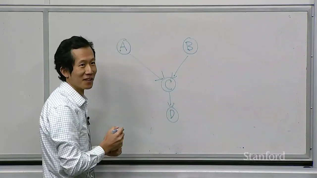
Two things follow that are easy to miss. First, the number of places you can end up now exceeds the number of choices you have. Second, that failed-tram branch is a self-loop, so the graph has cycles, which last week's machinery would have choked on. He waves this off — the algorithms to come handle cycles without complaint — and moves on.
 

A student asked where the probabilities come from. The answer is slightly deflating and worth knowing: they're part of the problem statement, and he just made up 0.4. In general you'd estimate them, or use reinforcement learning, which doesn't require knowing them at all. That's Wednesday's topic.
 

The rest of the section translates the code into notation. Actions(s) is the action set; Reward(s,a,s′) is what you collect if you take a from s and land on s′; T(s,a,s′) is the chance of that landing. There's a nice framing buried here: the triple packs in two decisions, yours (s to a) and nature's (a to s′), and you only control the first. Then the sanity check — for every state-action pair, the outgoing probabilities must sum to one, so at every dashed "chance node" on his diagram, 0.4 plus 0.6 is 1.
 

The comparison with search problems gets stated cleanly near the end. States, actions, start state, end test, successor function: all shared. Costs versus rewards: cosmetic. The real difference, in his words, is that a search action has one next state while an MDP action has a distribution over next states — and that difference is the reason this lecture exists.
 

Policies, Rollouts, and How Much the Future Is Worth

 

Here's where the consequences start landing. Under uncertainty, a solution can't be a fixed list of moves, because where you end up changes what's even available next. So the solution becomes a policy: a map from states to actions. Whatever happens to you, you consult the policy and it tells you what to do.
 

He shows two toy policies on the tram problem. Always-walk ignores the state entirely and returns walk every time. Tram-if-possible takes the tram while doubling keeps you in bounds, which means at state 6 and beyond you're forced to walk, since 12 overshoots 10.
 

To judge a policy you roll it out: simulate it against the MDP, with the policy choosing actions and the MDP sampling the outcomes according to its probabilities. Each rollout produces a sequence of steps, and the utility of that sequence is a discounted sum of rewards.
 

The discount gets a full treatment, and honestly it needed one, because it's the first genuinely new knob. Gamma equals 1 means no discounting — the future counts as much as the present. Gamma equals 0 wipes out everything except the first reward; in the walking demo that collapses the utility to −1. Gamma at 0.5 means each further step is worth half the one before, which he illustrates with the money version: a dollar today is worth fifty cents tomorrow.
 

The question period around this is better than most lecture Q&A. Someone asked whether the power form of discounting is the only option — it's the only one in this class, chosen partly because it's convenient for certain algorithms, and he offers to discuss alternatives offline. Someone else asked why bother discounting at all. His answer: if your policy needs a long reasoning chain before it produces anything, you want gamma close to 1, maybe 0.99. Heavy discounting isn't just "I don't care about later," it functions as a mild penalty on taking longer. Someone else pressed on why reward is defined over (s, a, s′) rather than over states alone — all the variants are essentially equivalent, since you can absorb the dependence by inserting dummy states, and he prefers the richer form because it's more natural to write down and costs nothing algorithmically.
 

Then the payoff: run the same policy twice and you get different utilities. With randomness in the transitions, there are exponentially many things that can happen.
 

Monte Carlo Policy Evaluation and Its Square-Root Ceiling

 

So how do you score a policy if a single run tells you nothing? You average. The value of a policy, written V^π(s), is the expected utility of rollouts that start at s and follow π from then on. He generalizes to arbitrary starting states on purpose, and notes that anyone who remembers dynamic programming from last week should be hearing an echo of future cost. It isn't quite future cost, but it's the same move: attach a number to a state that summarizes everything downstream.
 

The naive implementation is Monte Carlo policy evaluation — run N rollouts, collect N utilities, take the mean. For a deterministic policy like always-walk, one rollout is enough, and he uses that as the teaching point rather than reading a number off the screen. I found the omission slightly annoying; by my own count walking from 1 to 10 should be nine steps at −1 each, but he never says it out loud.
 

Tram-if-possible with 20 rollouts comes out around −11.7. Push N up and the estimate tightens. Then the rate: error shrinks roughly like one over the square root of the number of rollouts, so a hundred rollouts buys you about a tenth. His own verdict is that this isn't terrible, but "we're going to see that we can do a lot better."
 

This is also where the lecture hit its roughest patch for me. A student kept pushing on why the average converges to a single number when the outcomes themselves never settle — if a coin keeps alternating heads and tails, where does the fixed value come from? He reaches for the coin-flipping analogy: individual flips don't converge, but the fraction of heads does, and that fraction is what you're estimating. The distinction is between a random variable and its expectation, and the analogy is the right one, but the student didn't look satisfied and the exchange ended with "I'm happy to address that later." I'd have spent another thirty seconds there.
 

The dice game is the entertainment break, and it lands. Each round you quit and take $10, or stay, collect $4, and let him roll a die: a one or a two ends the game, anything else sends you to the next round. Quitting is deterministic and worth exactly 10, one rollout, done. Staying with 20 rollouts produces a scatter of 4s, 8s, the occasional 60 when someone gets absurdly lucky, and an average around 12.8 against quitting's 10. He polls the room, people stick with quitting, he laughs and says they clearly don't trust the simulation.
 

The general lesson is small but genuine: if you're choosing between two candidate policies, estimating both values and comparing is enough. The catch is that they're only estimates, which is exactly what sets up the rest of the hour.
 

Q-Values, Bootstrapping, and the Two-Phase Convergence Curve

 

Can the value be computed exactly rather than estimated? Yes, through a recurrence, and he's explicit that the skeleton is last week's future-cost recursion with probabilities grafted on.
 

The intermediate quantity is the Q-value: the worth of committing to action a in state s and then inheriting the value of wherever you land. Written out, it sums over every successor the chance of that successor times the immediate reward plus gamma times that successor's value. He mentions his three-argument version (state, action, value function) is a bit nonstandard. A student asked how this differs from the sampling approach, and the answer is crisp: before, you picked one branch and lived with the noise; here you look at all of them weighted by probability, so there's no sampling error at all.
 

Then comes bootstrapping, which is the conceptual heart of the lecture. You start with a value vector meaning "the value of stopping right now" — zero at the end state, and an admittedly arbitrary −100 everywhere else, standing in for "I haven't figured out how to get anywhere from here." One iteration later, the vector means "follow the policy for one step, then stop." Two iterations, "follow for two steps, then stop." You keep feeding the vector back into the recurrence until it stops changing.
 

The stopping rule is worth writing down: compare successive vectors element-wise, take the largest absolute difference (the L-infinity distance), and quit when it drops below 1e-5. Taking the maximum rather than an average matters, because otherwise one well-converged state can mask another that's still wildly off.
 

The worked arithmetic is where this clicked for me. State 9 updates to −1, because the only legal move is a one-minute walk into the end state. State 5 lands near −42, and the reason is instructive: 60% of the time the tram fires and costs you 2, 40% of the time you go nowhere and you're still holding that −100 placeholder. The states where only walking is available come out as clean integers with no decimals, which is a neat visual tell for where the randomness is. The full run converges in 27 iterations to roughly −12.5 — he reads it out as "minus twelve" — against the −11.7 Monte Carlo estimate. The dice game, with only two states, converges to exactly 12 against the 12.8 estimate.
 

His reading of the convergence curve is the most interesting aside in the lecture. The distance sits pinned near 100 for a while, then decays exponentially. There are two phases: the first is pure reachability — from state 1 you simply cannot reach state 10 in a handful of steps, so no amount of iterating helps — and only once every state has a real path out does the refinement phase begin, and that part decays exponentially.
 

Value Iteration and the Loose Ends Left at the Bell

 

With about ten minutes left he admits he still hasn't told anyone how to actually solve an MDP, makes a joke at his own expense about time management, and then points out that almost no new work is required. Policy evaluation asks what a given policy is worth. Value iteration asks what the best policy is worth, and hands you the optimal policy as a byproduct. He notes this should feel suspicious — evaluating a function is usually trivial while finding its minimizer can be intractable — and credits Richard Bellman's dynamic programming work from the 1950s for why it works out here.
 

The modification is smaller than you'd expect. Where policy evaluation plugs in the action the policy dictates, value iteration takes the maximum over the available actions. Compute every Q-value for a state, take the max for the value and the argmax for the policy, and you're done. The initialization, the loop over states, and the L-infinity convergence check carry over untouched. He'd advertised this as a four-character change on a previous slide and then conceded it's more like one line.
 

On the flaky tram, the optimal value comes out at −7.3, comfortably better than the −12-ish of tram-if-possible and better than walking. The optimal policy is a threshold rule: walk until you reach state 5, then start trying the tram. His intuition is that an unreliable two-minute tram isn't worth gambling on early, but from state 5 onward a success jumps you far enough, and you get several attempts for that 0.6 to come up. He's careful to say the answer shouldn't feel obvious in general, which is the whole argument for having algorithms.
 

A good closing question: is the optimal policy always deterministic? For MDPs, yes — the value is a max, so some single action attains it, and a randomized policy could at best tie. He adds the teaser that this stops being true for games next week, where randomness genuinely helps.
 

Three things I left wanting. The dice game poll produced a promise that he'd explain why a hybrid strategy — stay a few rounds then quit — can't beat the pure options; as far as I can tell he never returns to it, and the intuition (the state never changes, so it's the same decision every round) is left for you to reconstruct. Second, the −100 initialization is called arbitrary, and it visibly manufactures that two-phase convergence curve, but he never says whether your starting values change where the iteration ends up — they don't under the right conditions, but "contraction" never comes up, and neither do the conditions on gamma that make convergence safe. That matters more than it sounds, because the demos run with a discount of 1 on a graph with cycles, and convergence is asserted rather than argued. Third, the gap between the noisy estimates and the exact answers — −11.7 against −12.5, 12.8 against 12 — is a great accidental lesson in how little twenty rollouts buys you, and it's a shame the classroom vote was being decided on numbers that soft.
 

His parting advice is the one thing I'd write on the wall: study the recurrences and understand why they work, rather than memorizing the algorithms as procedures. Next week the transitions and rewards stop being given, and the whole problem turns into reinforcement learning.
 

Come away from this one knowing the shape of the thing — Markov decision processes turn a plan into a policy, a run into an expectation, and a one-off evaluation into a bootstrapped recurrence — and you'll be in good shape for Wednesday.
 

Content Disclaimer:

This article is for general reference only and does not constitute professional R&D guidance, production process advice or quality certification. All material performance data has specific test premises; readers should verify parameters against actual equipment and working conditions.