Stanford CS221 |Autumn 2025| Lecture 9: Policy Gradient — Annotated Lecture Notes & Key Takeaways

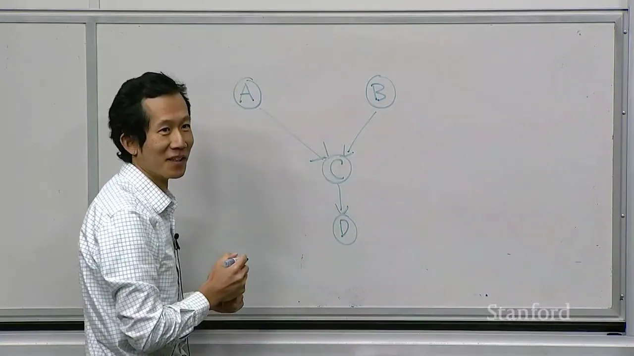
Course Information

Institution: Stanford

Original Course: Stanford CS221 | Autumn 2025 | Lecture 9: Policy Gradient

Instructor Bio: This lecture is delivered by Percy Liang, Associate Professor of Computer Science at Stanford University and core faculty of the Stanford Institute for Human-Centered Artificial Intelligence (HAI). Percy Liang leads the Stanford Natural Language Processing Group and the Center for Research on Foundation Models (CRFM). His research spans the theoretical foundations and practical systems of artificial intelligence, including machine learning, natural language processing, AI alignment, and rigorous model evaluation. He received his PhD in Computer Science from the University of California, Berkeley and his BA in Mathematics from Harvard University. His work has been recognized with the NSF CAREER Award, Google Faculty Research Award, and multiple best paper awards at top-tier AI conferences. He has taught CS 221 at Stanford for over a decade, shaping foundational AI education for thousands of students.

Course Description: This lecture dives into policy gradient methods, a major class of reinforcement learning algorithms that directly optimize parameterized policies rather than value functions. It covers the policy gradient theorem, the REINFORCE algorithm, and variance reduction techniques including advantage functions and actor-critic architectures. The lecture also discusses why policy gradient methods are particularly well-suited for high-dimensional state spaces and continuous action domains.

If you missed this session, here's the shape of it. The lecturer spends the first chunk mopping up the previous lecture — MDPs, Q-learning, SARSA — and then spends the remaining hour building policy gradient​ from the ground up: methods that adjust a policy directly rather than learning a value function and reading a policy off it. He opens by saying that by the end you should have the ingredients to read essentially any cutting-edge RL algorithm, and the whole talk is staged as a slow escalation toward that promise. It's a two-lecture RL block; this is the second one.
 

The Recap, and the Grid Everything Sits On

 

Reinforcement learning, he insists early, is more of a setting than an algorithm. Agent takes actions, environment returns rewards and observations, and the agent is supposed to make sense of that stream and pick better actions next time. What I appreciated about the framing is how much weight he puts on the isolation: the algorithm never sees the MDP. It only ever gets called with two things — a request for an action at a state, and a chunk of feedback about what happened. That's the entire window onto the world.
 

The running example is the "flaky tram" MDP. You start at location one and want location six; walking moves you from i to i+1, the tram jumps you from i to 2i but fails ten percent of the time. Walking costs −1, the tram costs −2. A concrete rollout he traces: walk to two, walk to three, tram to six, rewards −1, −1, −2, and with a discount of one the utility of that episode is −4. Run twenty rollouts and average the utilities and you've got a rough measure of how good the algorithm currently is against that MDP.
 

He then re-pins four quantities on the board. There's V^π(s), the expected utility of following policy π from state s; Q^π(s,a), the value of taking action a first and then following π; and then the starred versions where the policy in question is the optimal one. The Q values live on the chance nodes of the MDP tree, the V values on the state nodes.
 

From there he lays out the dimensions that organize the previous lecture's algorithms. Model-based means you estimate transitions and rewards first, then run value iteration. Model-free means you skip the MDP and go straight at Q values, then derive the policy by taking the action with the highest Q — going from Q to policy is easy, getting Q in the first place is the hard part. On-policy means the policy generating your data is the same one you're trying to evaluate; off-policy means you're learning about a different policy than the one you're behaving according to. And separately, full rollouts versus bootstrapping — waiting until the episode ends to get a real number, or cutting it short and plugging in your current estimate of what happens next.
 

Those axes give you the four algorithms: model-based value iteration, model-free Monte Carlo, SARSA, and Q-learning. The general update shape across the value-based ones is simple — you get a target, which is a noisy estimate of what Q should be, and you nudge your current Q toward it by an amount set by the learning rate.
 

A student asked when you'd pick SARSA over Q-learning. The answer was honest: it depends on the application. But the real distinction is that off-policy lets you explore aggressively while still guaranteeing you're estimating the optimal policy, whereas SARSA forces you to behave closer to the policy you're evaluating, or you end up evaluating the wrong thing. He tied it back to the earlier policy-evaluation-versus-value-iteration distinction: one takes the single action the policy dictates, the other takes a max.
 

When Lookup Tables Stop Working

 

Around the seventeen-minute mark the lecture turns. Storing a Q value for every state-action pair is fine in a toy MDP, but a robot's state might be an image and a language model's "state" might be a whole paragraph with the action being the next token. You cannot index a dictionary by an image.
 

A student suggested reducing the state space, and the lecturer partly agreed — you definitely have to compress somehow — but said he wanted to go at the problem more directly. That direct approach is function approximation: parameterize Q by some θ, map the state-action pair into a feature vector, and let a linear model or an MLP turn that vector into a single number. This is the point where the machine learning half of the course stops being a separate module and gets bolted onto the RL skeleton. He explicitly says to think of the architecture as a slot where you drop in whatever model you like.
 

The demo is deliberately humble: parameterized Q-learning on the same tram MDP, with one-hot features over all twelve state-action pairs. That choice makes the machine learning version mathematically equivalent to the tabular version, so it works as a sanity check rather than a showcase. Action selection stays ε-greedy. Feedback handling computes a target as the immediate reward plus the discounted Q of the next state under the current greedy action, defines a squared loss between prediction and target, and takes an SGD step.
 

Then the demo didn't work. After a hundred simulated runs, the learned Q values were, in his words, doing something reasonable but noticeably off, and the extracted policy wasn't the walk-walk-walk-then-tram solution it should have been. He chalked it up to an unlucky random run and noted a previous execution had found the optimal policy. As a listener I found this the weakest moment in the first half. A demo whose entire purpose is to verify that the machinery reproduces a known answer, and which then fails to reproduce it, needs more than "run it longer and it should be fine."
 

Two questions followed that were more interesting than the demo. First: why squared error? The reasoning is that a target is a noisy proxy for the quantity you actually want — with Monte Carlo targets, averaging a million rollouts would converge on the true value — so regressing onto individual targets is just standard regression pulling your estimate toward those samples. Second: does this converge? In the tabular case, yes under conditions like exploring everywhere. With function approximation, he said flatly, there are no general guarantees; you might show convergence to a local optimum, which is less exciting. That's a striking admission and he moves past it in about fifteen seconds. I wanted the intuition for why approximation breaks the tabular guarantee, and it never came.
 

Building Policy Gradient from Scratch

 

The pivot at about 34:20 is a nice rhetorical move. Model-based methods estimate the MDP. Value-based methods estimate Q. But if what you ultimately want is a policy, why estimate Q at all? He even asks whether he's been wasting everyone's time. He's not, but the question sets up the rest.
 

A policy, reframed, is just a classifier: state in, action out. The problem is that classifiers are hard to optimize directly because the zero-one loss has zero gradient nearly everywhere. The fix is the same one from the machine learning lectures — make it probabilistic. Now the policy outputs a distribution over actions, which is continuous and therefore differentiable.
 

Before the math he detours through imitation learning (~36:30). If an expert hands you demonstrations — someone teleoperating a robot arm to pick up a cup, or people hired to write out worked solutions to math problems — you don't need RL at all. You maximize the log probability of the demonstrated action at each state and go home. The catch is that the RL environment only ever gives you reward, never the right answer.
 

So the move is to imitate yourself. Roll out your current policy, and you'll get some good trajectories and some bad ones. Weight each one by how good it turned out to be, and do imitation learning on the result. He offers this as the zeroth-order version of what's coming, and it's a genuinely useful anchor to hold onto through the algebra.
 

The formal setup: a trajectory τ is a sequence of state, action, reward, state, action, reward, ending in a state. By the chain rule, the probability of a trajectory under parameters θ is an alternating product of policy terms and environment transition terms — your action choices interleaved with the world's responses. The initial state is deterministic so it contributes nothing.
 

Then the objective, which he presents as the most direct possible statement of what RL is trying to do: maximize the expected utility of a trajectory, where the expectation is over trajectories weighted by their probability under your current policy. No MDPs, no Q values, just expected utility.
 

The derivation that follows is the technical heart of the lecture and also the densest part. You take the gradient of that expectation, expand it into an explicit sum over trajectories, push the gradient inside the sum, and then apply what he calls the log-gradient identity — the gradient of a probability can be rewritten as that probability times the gradient of its log. The reason for the rewrite is structural: it puts a probability factor back in front, which lets you fold the whole sum back up into an expectation. And an expectation you can't compute can be approximated by sampling. Sample one trajectory, and your update direction becomes the gradient of the log-probability of that trajectory multiplied by its utility.
 

He's charmingly dismissive about the name here, saying it's called the policy gradient theorem but it's elementary enough that he'd just call it an identity and doesn't think it deserves to be called a theorem.
 

Unpacked over time steps, the gradient becomes a sum of per-step log-probability gradients, all multiplied by the utility of the whole episode. This is REINFORCE, which he attributes to Williams 1992 as the earliest and simplest instance of the general class. The intuition maps cleanly onto the earlier imitation-learning framing: maximize the probability of what you actually did, weighted by how good it was. If utilities are only zero or one, this is exactly imitation learning on the successful rollouts. If a trajectory scored badly, the weight flips and you push its probability down.
 

The Implementation, and the Multiplier That Went Missing

 

The code walkthrough starts around 54:00. The model is now a matrix mapping a one-hot state vector to logits over actions, because it's a multiclass classifier. Action selection computes logits, applies a softmax, and samples from the resulting distribution. Worth noting: there's no separate exploration policy anymore. The stochastic policy does the exploring by itself, which he flags as a genuine simplification, though you could add more exploration on top if you wanted.
 

Feedback handling accumulates the whole episode and only updates at the end, exactly like Monte Carlo, because you need the total utility before you can weight anything. At the terminal state, it walks back through each step, computes cross-entropy between the logits and the action actually taken, sums those up, and takes a gradient step.
 

Except — and this is where I got genuinely confused — he never multiplies the accumulated loss by the utility. He catches it on the spot, says the loss should be scaled by the utility, acknowledges he didn't do it, and then observes that the algorithm seems to have worked anyway. It did, in the sense that the learned policy came out as walk, walk, tram, walk, walk across the states, which looks about right.
 

But that's precisely the problem. The entire conceptual payload of REINFORCE is the utility weighting; without it you're doing plain imitation learning on your own rollouts, reinforcing whatever you happened to do regardless of outcome. If that still produces a sensible policy on this MDP, something about the example is doing the work — maybe every action sequence terminates quickly so there's little room for a bad policy to be much worse than a good one — but he doesn't explain it. For a listener trying to watch the central mechanism actually function, having it silently disabled and then shrugged off is the most frustrating thirty seconds in the lecture.
 

A couple of audience questions close the section. Someone asked about initialization, and the answer is that it matters more here than in ordinary supervised learning: your initial policy determines what data you collect, so a bad start starves you of useful experience. Small initial weights giving a near-uniform action distribution are the safe default. Another asked about online versus batched updates; the spirit is online, though you can batch rollouts to make it look more offline.
 

Variance, Baselines, and the Bridge to Actor-Critic

 

The last big block (~1:01) is about making that sampled gradient estimate less noisy, and the payoff is a control-variate idea borrowed from statistics.
 

He sets it up with a toy problem: estimating the mean of a small set of numbers. An estimator is just any random variable that tries to land near the target. Draw a single index and return its value and you're unbiased, but the variance is high — around 36 on his example. Average two samples and the mean stays put while the variance drops. Add random noise and you stay unbiased but get worse. Then the trick: subtract some offset function whose mean is zero. Linearity of expectation means the expected value is untouched, but the variance can fall dramatically. On his numbers it collapsed.
 

His explanation for why that works is worth holding onto: values sitting far below the mean get pulled up, values far above get pulled down. Any prior knowledge you have about roughly where the mean sits relative to your samples can be converted into variance reduction. (Small aside: the probabilities on his example slide didn't quite sum to one and he asked the room to "just imagine" they were a quarter each. Harmless, but noticeable if you were following the arithmetic.)
 

Ported back to RL, the offset becomes a baseline: any function of the state that doesn't depend on the action. He claims without full proof that the expected product of the log-policy gradient and such a baseline is zero, which means you can subtract it from the utility without biasing your gradient estimate while potentially cutting variance a lot. He draws an explicit analogy to A* search, where a heuristic encodes domain knowledge about future cost and speeds everything up; a good baseline plays the same role here.
 

Then, in the interest of time, he skips the proof and asks the room to trust him. I'd have traded five minutes of something else for it. The identity is the kind of thing that feels like sleight of hand until you see the cancellation, and it's load-bearing for the rest of the section.
 

He then lists two more modifications without developing them. You can replace the full-episode utility at each step with the rewards from that step onward, since what already happened can't be affected by what you do now. And you can swap the sampled utility for a bootstrapped estimate of the value function — which brings Q values back through the side door and gives you actor-critic methods, where a value function and a policy are learned simultaneously and can even share parameters in a deep network. The closing framing is a trade-off: baselines reduce variance while staying unbiased, bootstrapping reduces variance at the cost of introducing bias.
 

Where I Came Away Unsure

 

Three things stuck with me as unresolved. The failed Q-learning demo, dismissed as bad luck. The missing utility multiplier in REINFORCE, which quietly removed the mechanism the lecture was built to demonstrate and was never explained. And the skipped baseline proof sitting next to the unsupported claim that function approximation voids convergence guarantees — both are places where the argument would benefit from another pass.
 

There's also a quieter gap. The framing of a policy as a classifier assumes a discrete action set, but the motivating example for function approximation was a robot whose actions are continuous joint commands. The lecture never says how the distribution-over-actions trick extends there.
 

The final summary (~1:12:50) is genuinely clarifying, though. Three families — model-based, value-based, policy-based — and all of them share one skeleton: roll out using some exploration policy, write down a loss over some parameters, take a gradient step. The parameters belong to the MDP in one case, the Q function in another, the policy in the third. That reframing is what makes the lecture's opening promise feel earned rather than rhetorical.
 

He closes by teasing what's next: environments with adversaries, where you can't take expectations anymore and have to reason about worst cases. Which sounds like game theory is about to land on top of everything above.
 

Back to where we started — the reason policy gradient​ matters here isn't that it beats Q-learning on a six-state tram problem. It's that it's the formulation that survives contact with large or continuous action spaces, and it's the substrate that actor-critic methods and most of modern deep RL are built on. If you only take one thing from the hour, take the sampled objective: log-probability of what you did, times how well it went.
 

Content Disclaimer:

This article is for general reference only and does not constitute professional R&D guidance, production process advice or quality certification. All material performance data has specific test premises; readers should verify parameters against actual equipment and working conditions.