Deep Reinforcement Learning: Lecture 3 Policy Gradients Structured Notes & In-Depth Analysis

One. Course Details

This is the third lecture of Stanford University's CS224R Deep Reinforcement Learning course, taught by Professor Chelsea Finn. It transitions from offline imitation learning to online reinforcement learning—the core paradigm that allows agents to improve through trial and error—and introduces policy gradients, the first and most fundamental online RL algorithm covered in the course.
The lecture covers the full mathematical derivation of vanilla policy gradients (the REINFORCE algorithm), the intuitive interpretation of how policy gradients work, key limitations (especially high variance), and practical techniques to address these limitations. It also introduces the critical distinction between on-policy and off-policy algorithms and derives an off-policy variant of policy gradients using importance sampling. Policy gradients form the foundation of many state-of-the-art RL systems, including those used to train legged robots and fine-tune large language models.
The core goal of this lecture is to equip students to not only understand the theory behind policy gradients but also implement them correctly, diagnose common failure modes, and apply appropriate variance reduction techniques for real-world tasks.

Two. Key Learning Objectives

By the end of this lecture, students should be able to:

1. Describe the standard iterative loop of all online reinforcement learning algorithms
2. Derive the vanilla policy gradient formula using the log-derivative trick
3. Explain the intuitive meaning of policy gradients as weighted imitation learning
4. Implement two core variance reduction techniques: future reward weighting and baseline subtraction
5. Define the difference between on-policy and off-policy reinforcement learning
6. Use importance sampling to derive an off-policy policy gradient estimator
7. Identify the strengths, weaknesses, and optimal use cases for policy gradient methods

Three. Memorable Course Quotes

• "Policy gradients formalize the trial-and-error learning process: do more of what works and less of what doesn't."
• "The biggest challenge with policy gradients is not the math—it's the high variance of the gradient estimates."
• "Subtracting a baseline doesn't change the expected gradient, but it can drastically reduce its variance."
• "On-policy algorithms require you to throw away all your data after every gradient step—this is their biggest practical limitation."
• "Policy gradients work best with dense reward signals and large batches of data; they struggle mightily with sparse rewards."

Four. Detailed Study Notes

4.1 The Online Reinforcement Learning Loop

All online RL algorithms follow the same basic iterative process, which distinguishes them from offline methods like imitation learning:

1. Initialize the policy: This can be done randomly, with imitation learning weights, or using hand-designed heuristics. Initializing with expert demonstrations is almost always better than random initialization for complex tasks.
2. Collect data: Run the current policy in the environment to collect a batch of trajectories (rollouts).
3. Improve the policy: Use the collected data to update the policy parameters to increase expected future reward.
4. Repeat: Discard the old data, collect new data with the updated policy, and continue iterating.

This loop allows agents to learn from their own experience and potentially outperform any expert demonstrator, a capability that offline imitation learning lacks.

4.2 Vanilla Policy Gradient (REINFORCE) Derivation

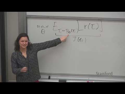
The goal of reinforcement learning is to maximize the expected sum of rewards over trajectories generated by the policy π_θ: J(θ) = E_{τ ~ p_θ(τ)} [r(τ)] where r(τ) is the total reward of trajectory τ and p_θ(τ) is the probability distribution over trajectories induced by policy π_θ.
To optimize this objective using gradient ascent, we need to compute ∇_θ J(θ). Direct differentiation is impossible because we cannot differentiate through the environment dynamics or the sampling process. Instead, we use the log-derivative trick:

1. Rewrite the expectation as an integral: J(θ) = ∫ p_θ(τ) r(τ) dτ
2. Bring the gradient inside the integral: ∇_θ J(θ) = ∫ ∇_θ p_θ(τ) r(τ) dτ
3. Apply the identity ∇_θ p_θ(τ) = p_θ(τ) ∇_θ log p_θ(τ): ∇_θ J(θ) = ∫ p_θ(τ) ∇_θ log p_θ(τ) r(τ) dτ
4. Convert back to an expectation: ∇_θ J(θ) = E_{τ ~ p_θ(τ)} [∇_θ log p_θ(τ) r(τ)]

Next, we decompose the trajectory probability p_θ(τ): p_θ(τ) = p(s₁) ∏ₜ=₁^T π_θ(aₜ | sₜ) p(sₜ₊₁ | sₜ, aₜ)
Taking the log and then the gradient eliminates the initial state distribution and environment dynamics terms, which do not depend on θ: ∇_θ log p_θ(τ) = ∑ₜ=₁^T ∇_θ log π_θ(aₜ | sₜ)
Substituting back gives the final vanilla policy gradient formula: ∇_θ J(θ) = E_{τ ~ p_θ(τ)} [ (∑ₜ=₁^T ∇_θ log π_θ(aₜ | sₜ)) * r(τ) ]
This is the REINFORCE algorithm. In practice, we estimate this expectation using a batch of sampled trajectories.

4.3 Intuitive Interpretation of Policy Gradients

Policy gradients can be understood as weighted imitation learning:

• The term ∇_θ log π_θ(aₜ | sₜ) is exactly the same gradient used in imitation learning. It pushes the policy to increase the probability of taking action aₜ in state sₜ.
• The total trajectory reward r(τ) acts as a weight. If the trajectory had a high reward, we increase the probability of all actions taken in that trajectory. If the trajectory had a low reward, we decrease the probability of all actions taken in that trajectory.

This directly formalizes the trial-and-error learning process: agents repeat behaviors that lead to good outcomes and avoid behaviors that lead to bad outcomes.

4.4 The High Variance Problem

Vanilla policy gradients produce extremely noisy gradient estimates, which is their biggest limitation. This noise arises because we are estimating an expectation using a finite number of samples. Small changes in the sampled trajectories can lead to drastically different gradient estimates.

4.4.1 First Variance Reduction Technique: Future Reward Weighting

The vanilla gradient incorrectly weights actions by the total trajectory reward, including rewards that occurred before the action was taken. Since actions cannot affect the past, we should only weight each action by the future rewards it can influence: ∇_θ J(θ) = E_{τ ~ p_θ(τ)} [ ∑ₜ=₁^T ∇_θ log π_θ(aₜ | sₜ) * (∑ₜ'=ₜ^T r(sₜ', aₜ')) ]
This simple change significantly reduces variance and makes the gradient more accurate. For example, if an agent takes a bad step early but recovers and gets a high reward later, the bad early step will be correctly penalized instead of rewarded.

4.4.2 Second Variance Reduction Technique: Baseline Subtraction

Another major source of variance is the absolute scale of the reward function. If all rewards are positive, the policy will try to increase the probability of all actions, even those from below-average trajectories.
We can fix this by subtracting a baseline b from the reward term: ∇_θ J(θ) = E_{τ ~ p_θ(τ)} [ ∑ₜ=₁^T ∇_θ log π_θ(aₜ | sₜ) * (∑ₜ'=ₜ^T r(sₜ', aₜ') - b) ]
Crucially, subtracting a constant baseline does not change the expected value of the gradient. This can be proven mathematically by showing that E[∇_θ log p_θ(τ) * b] = 0.
The most common and effective baseline is the average reward of the current batch of trajectories. This ensures that actions from above-average trajectories are encouraged and actions from below-average trajectories are discouraged, regardless of the absolute reward scale.

4.5 On-Policy vs. Off-Policy Learning

Policy gradients as derived are on-policy algorithms, meaning the gradient estimate requires data collected from the exact current policy π_θ. This means we must discard all data after taking a single gradient step, which is extremely data-inefficient.
In contrast, off-policy algorithms can reuse data collected from any previous policy, making them much more data-efficient.

4.6 Off-Policy Policy Gradients with Importance Sampling

We can derive an off-policy variant of policy gradients using importance sampling, a statistical technique for estimating expectations under one distribution using samples from another distribution.
If we have samples from an old policy π_θ_old and want to estimate the expected reward under a new policy π_θ_new, we weight each sample by the importance ratio: w(τ) = p_θ_new(τ) / p_θ_old(τ)
The off-policy policy gradient then becomes: ∇_θ J(θ) = E_{τ ~ p_θ_old(τ)} [ w(τ) * ∇_θ log p_θ_new(τ) * r(τ) ]
In practice, the trajectory-wise importance ratio can become numerically unstable for long trajectories because it involves multiplying many small probabilities together. A common approximation is to use per-time-step importance ratios instead.
This allows us to take multiple gradient steps on a single batch of data, significantly improving data efficiency.

4.7 Practical Implementation Notes

• Surrogate Objective: Instead of computing the gradient directly, we can define a surrogate objective whose gradient equals the policy gradient. This allows us to use standard automatic differentiation libraries with a single forward and backward pass: L(θ) = E_{τ ~ p_θ(τ)} [ ∑ₜ=₁^T log π_θ(aₜ | sₜ) * (∑ₜ'=ₜ^T r(sₜ', aₜ') - b) ]
• Batch Size: Policy gradients require large batch sizes to reduce variance. Small batches will produce extremely noisy gradients and may fail to learn entirely.
• Reward Denseness: Policy gradients work best with dense reward signals. Sparse rewards (e.g., only 1 for success and 0 for failure) lead to very slow learning or no learning at all.
• These are my structured study notes and in-depth interpretations compiled by watching the open course. I hope this knowledge framework helps you master the content of this subject thoroughly. Wish you continuous academic progress and great achievements in your studies.