One. Course Details
This is the fourth lecture of Stanford University's CS224R Deep Reinforcement Learning course, taught by Professor Chelsea Finn. It builds directly on the policy gradient methods introduced in Lecture 3 and presents actor-critic algorithms—the most widely used family of deep RL algorithms in practice, which form the foundation for state-of-the-art methods like PPO used to train large language models and humanoid robots.
The lecture covers the mathematical definition and intuitive interpretation of value functions, Q-functions, and advantage functions, three core techniques for policy evaluation (Monte Carlo estimation, temporal difference learning, and n-step returns), and the complete end-to-end actor-critic algorithm pipeline. A key focus is on how actor-critic methods address the high variance and poor data efficiency limitations of vanilla policy gradients by learning an explicit estimate of future rewards.
The core goal of this lecture is to equip students to understand the theory behind actor-critic methods, implement them correctly, and make informed trade-offs between bias and variance when estimating value functions for real-world tasks.
Two. Key Learning Objectives
By the end of this lecture, students should be able to:
- Define and distinguish between value functions (V), Q-functions (Q), and advantage functions (A)
- Explain the mathematical relationship between V, Q, and A
- Describe three methods for policy evaluation and compare their bias-variance trade-offs
- Derive the actor-critic policy gradient using the advantage function
- Implement the complete actor-critic algorithm with separate actor and critic networks
- Explain how bootstrapping works in temporal difference learning and its benefits
- Apply discount factors and n-step returns to improve value function estimation
Three. Memorable Course Quotes
- "Policy gradients don't always make efficient use of the data we've collected. If we can figure out what actions are advantageous versus not, we can make much better use of that data."
- "Actor-critic methods learn to estimate what's good and bad, then do more of the good stuff according to your estimate."
- "Monte Carlo estimation has high variance but is completely unbiased. Bootstrapping has much lower variance but can be biased by the quality of your current value estimate."
- "The advantage function tells you exactly how much better taking a particular action is than following your average policy in that state."
- "Actor-critic algorithms have two separate neural networks: the actor that decides what to do, and the critic that tells the actor how good its decisions were."
Four. Detailed Study Notes
4.1 Recap: Limitations of Vanilla Policy Gradients
Before introducing actor-critic methods, Professor Finn recaps the key limitations of the policy gradient algorithms covered in the previous lecture:
- High variance: Gradient estimates are based on single trajectory returns, leading to noisy updates
- Poor data efficiency: On-policy nature requires discarding all data after one gradient step
- Inefficient credit assignment: All actions in a trajectory are weighted by the total return, even if some actions were good and others were bad
For example, if a robot takes a small step forward but then falls backward, vanilla policy gradients will penalize the forward step because the total trajectory return is negative, even though the step itself was progress toward the goal. Actor-critic methods solve this problem by learning an explicit estimate of how good each state and action is.
4.2 Core Value Function Concepts
Actor-critic methods rely on three fundamental quantities to evaluate policies:
4.2.1 Value Function (V^π(s))
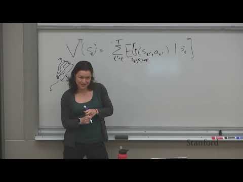
The value function of a state
s under policy π is the expected sum of future rewards the agent will receive if it starts in state s and follows policy π for all subsequent steps: V^π(s) = E_{τ ~ π | s₀=s} [Σₜ'=ₜ^T r(sₜ', aₜ')]Intuitively, it answers the question: "How good is it to be in this state right now if I follow my current policy?"
4.2.2 Q-Function (Q^π(s, a))
The Q-function (or action-value function) of a state-action pair
(s, a) under policy π is the expected sum of future rewards the agent will receive if it starts in state s, takes action a, and then follows policy π for all subsequent steps: Q^π(s, a) = E_{τ ~ π | s₀=s, a₀=a} [Σₜ'=ₜ^T r(sₜ', aₜ')]It answers the question: "How good is it to take this specific action in this state right now?"
4.2.3 Advantage Function (A^π(s, a))
The advantage function measures how much better taking action
a in state s is compared to following the average policy π in that state: A^π(s, a) = Q^π(s, a) - V^π(s)This is the most important quantity for actor-critic methods. A positive advantage means the action is better than average; a negative advantage means it is worse than average.
4.2.4 Intuitive Example: Learning to Play Drums
To illustrate these concepts, Professor Finn uses a simple example:
- Reward: 1 if you can play drums in one month, 0 otherwise
- Actions: Sit on the beach, watch TV, practice drums
- Current policy: Always sit on the beach
For this scenario:
V^π(s) = 0(following the current policy will never lead to learning drums)Q^π(s, sit on beach) = 0,Q^π(s, watch TV) = 0Q^π(s, practice drums) ≈ 1(practicing once gives a chance to learn)A^π(s, practice drums) = 1 - 0 = 1(practicing is much better than the average policy)
4.3 Improving Policy Gradients with Advantage Functions
The vanilla policy gradient can be rewritten using the advantage function to produce a much more accurate and lower-variance gradient estimate:
∇_θ J(θ) = E_{τ ~ π_θ} [ Σₜ=₁^T ∇_θ log π_θ(aₜ | sₜ) * A^π(sₜ, aₜ) ]This is a significant improvement over vanilla policy gradients because:
- It only rewards actions that are better than average, rather than all actions in high-return trajectories
- It correctly penalizes actions that are worse than average, even in high-return trajectories
- It produces much lower-variance gradient estimates
The challenge now becomes how to accurately estimate the advantage function
A^π(s, a).
4.4 Policy Evaluation: Estimating Value Functions
To compute the advantage function, we first need to estimate the value function
V^π(s). There are three main methods for policy evaluation, each with different bias-variance trade-offs:
4.4.1 Monte Carlo Estimation
The simplest approach is to use the actual sum of future rewards observed in trajectories as the target for the value function:
- Target:
y_t = Σₜ'=ₜ^T r(sₜ', aₜ') - Training objective:
min_φ Σ ||V_φ(s_t) - y_t||² - Properties: Unbiased (uses actual observed returns) but high variance (each trajectory is a single sample from the distribution)
Monte Carlo estimation requires waiting until the end of each trajectory to compute the target, making it unsuitable for very long or infinite-horizon tasks.
4.4.2 Temporal Difference (TD) Learning (Bootstrapping)
TD learning addresses the high variance of Monte Carlo estimation by using bootstrapping—using the current estimate of the value function to compute the target:
- Target:
y_t = r(s_t, a_t) + V_φ(s_{t+1}) - Training objective:
min_φ Σ ||V_φ(s_t) - y_t||² - Properties: Low variance (only depends on one immediate reward and one value estimate) but biased (relies on the current, imperfect value function estimate)
TD learning can update the value function after every time step, making it much more efficient for long-horizon tasks. It propagates value information backward through time as the agent gains experience.
4.4.3 N-Step Returns
N-step returns provide a middle ground between Monte Carlo and TD learning by balancing bias and variance:
- Target:
y_t = Σₖ=₀^{n-1} r(s_{t+k}, a_{t+k}) + V_φ(s_{t+n}) - Properties: Lower variance than Monte Carlo, lower bias than 1-step TD
The choice of
n is a hyperparameter that controls the bias-variance trade-off. Smaller n gives lower variance but higher bias; larger n gives lower bias but higher variance. In practice, values between 5 and 20 often work best.
4.4.4 Discount Factors
For long or infinite-horizon tasks, we typically add a discount factor
γ (between 0 and 1) to weight immediate rewards more heavily than future rewards:
- Discounted n-step target:
y_t = Σₖ=₀^{n-1} γᵏ r(s_{t+k}, a_{t+k}) + γⁿ V_φ(s_{t+n})
Intuitively, this is equivalent to assuming there is a
1-γ probability that the episode will end at each time step. Discount factors prevent value estimates from becoming infinitely large and help stabilize training.
4.5 The Complete Actor-Critic Algorithm
Actor-critic algorithms use two separate neural networks:
- Actor network (π_θ): Maps states to actions (the policy)
- Critic network (V_φ): Maps states to value estimates (evaluates the policy)
The full algorithm follows this iterative loop:
- Sample trajectories: Run the current actor policy in the environment to collect a batch of trajectories
- Fit the critic: Train the critic network to predict value functions using either Monte Carlo, TD, or n-step targets
- Compute advantages: For each state-action pair, estimate the advantage function using
A(s_t, a_t) ≈ r(s_t, a_t) + γ V_φ(s_{t+1}) - V_φ(s_t) - Update the actor: Compute the policy gradient using the estimated advantages and update the actor network parameters
- Repeat: Discard the old data and collect new trajectories with the updated actor policy
4.6 Key Benefits of Actor-Critic Methods
- Lower variance gradients: Advantage function estimates produce much more stable updates than vanilla policy gradients
- Better credit assignment: Correctly identifies which actions are good or bad, rather than weighting all actions in a trajectory equally
- Higher data efficiency: Can take multiple gradient steps on the critic network for each batch of data
- Works well with sparse rewards: Can learn from partial progress toward the goal by estimating intermediate state values
- These are my structured study notes and in-depth interpretations compiled by watching the open course. I hope this knowledge framework helps you master the content of this subject thoroughly. Wish you continuous academic progress and great achievements in your studies.