Stanford CME296 Diffusion & Large Vision Models | Lecture 2 - Score matching — Annotated Lecture Notes & Key Takeaways

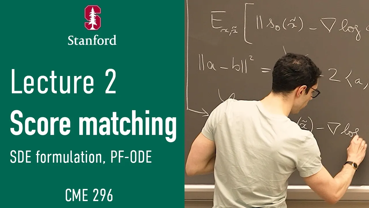
Course Information

Institution: Stanford

Original Course: Stanford CME296 Diffusion & Large Vision Models | Spring 2026 | Lecture 2 - Score matching

Instructor Bio: This lecture is co-delivered by **Afshine Amidi** and **Shervine Amidi**, adjunct faculty at Stanford University’s Institute for Computational and Mathematical Engineering (ICME). Afshine Amidi earned his engineering degree from École Centrale Paris and a Master of Science in Operations Research from the Massachusetts Institute of Technology, where he worked under Prof. Dimitris Bertsimas and received the Jean Gaillard Scholarship and MIT Dean’s Fellowship. He has held professional roles at Amazon and McKinsey & Company, leading AI and business strategy initiatives, and co-authors widely adopted technical learning guides on machine learning, algorithms, and transformer models. Shervine Amidi holds B.S. and M.S. degrees in engineering from École Centrale Paris, as well as an M.S. in Computational and Mathematical Engineering from Stanford University. He has conducted computer vision research at the Stanford Vision Lab and the École Centrale Paris Visual Computing Center. Currently a Senior Machine Learning Engineer at Netflix, he previously worked at Google DeepMind on the Gemini team, Google Assistant, and Uber’s data science division. He has served as a teaching assistant for multiple core Stanford CS courses and has been an adjunct lecturer at the university since 2021.

Course Description: This lecture introduces the theoretical framework of score-based generative modeling as an alternative perspective on diffusion-based generation. It covers the motivation for score estimation, denoising score matching techniques, the mathematical connection between score functions and Stochastic Differential Equations (SDEs), training and inference procedures for continuous-time score-based systems, and the probability flow ODE formulation that unifies diffusion and score-based generative approaches.

This is the second session of Stanford's CME 296, and it runs long — roughly an hour and forty-eight minutes, split between two instructors. The first hour or so is a ground-up construction of score matching​ as an alternative route to the same destination DDPM reached last week. The last stretch throws the discrete-time framing away entirely and rebuilds the whole thing in continuous time, then finishes with a sampler that exploits the new formulation. I'll flag up front that the lecture is unusually candid about what it is skipping: several derivations are explicitly deferred, and one of them is promised for next week.
 

Picking Up Where DDPM Left Off

 

The opening minutes are a reset, and they're worth taking seriously because the entire lecture is framed as "same goal, different derivation." The goal is unconditional generation: no input, no conditioning signal, just learn to produce new images from an unknown and possibly horrible data distribution.
 

Last week's strategy was to take clean training images, define a forward process Q that corrupts them progressively until you have essentially pure noise, then train a reverse process that predicts which noise to remove. The justification ran through maximum likelihood — maximize the probability the model assigns to training data — which turned out to be intractable, so the class derived a tractable lower bound instead. Expanding that bound produced a KL divergence between the thing you actually want to learn and the fixed forward process you defined yourself. Gaussians made it tractable. The endpoint was a plain squared-error regression against the noise you injected, with a network taking the corrupted image and the noise level as inputs.
 

One small note on the recap: the lecturer calls the bound the "elbow" formulation throughout, which is just ELBO spoken aloud. If that phrase confused you in the recording, that's all it is.
 

What Score matching Actually Trains You to Estimate

 

The new perspective starts from a picture. You have training images — the running example is teddy bears — drawn from an unknown distribution. The plan is the familiar one: start somewhere easy to sample, like Gaussian noise, then walk toward the regions where real images live.
 

Concretely, imagine a density over image space where darker shading means higher probability. Drop a point somewhere in a pale region. How do you move toward the dark region? The gradient of the density points uphill, so take it. That's the whole intuition, and the lecturer pauses to define what a gradient is for anyone rusty: for a scalar function over a multi-dimensional input, it's the vector of partial derivatives with respect to each dimension, and it points in the direction of steepest increase.
 

Then he breaks it. Two reasons you can't just use the gradient of the density:
 

Densities are normalized. The integral over the entire space has to equal one, which means there's a normalizing constant — he labels it Z — that requires summing or integrating over every point in a very high-dimensional space. Intractable. And if the density itself is intractable, its gradient is too.
 

Densities get vanishingly small. In regions with little data, the value can be tiny enough to cause numerical trouble.
 

The fix is to take the gradient of the log density instead. This quantity gets a name — the score — and it's the reason the lecture has the title it does. Three arguments are given for why it's a better object.
 

The logarithm turns the normalizing constant from a factor you must compute into a term that vanishes. Since Z doesn't depend on position, its gradient with respect to x is zero.
 

It points the same way. A one-line calculus identity says the gradient of log p equals the gradient of p divided by p, and dividing a vector by a positive scalar only rescales it. Direction preserved.
 

It's numerically better behaved. Where the raw gradient is tiny, the density usually is too, so the ratio doesn't collapse the way either quantity does on its own.
 

There's a clarification I appreciated, because it's the kind of thing that silently trips people up: the gradient here is with respect to x, position in space, not with respect to model parameters. Score sometimes means the parameter gradient in other contexts, and he wants that ambiguity closed before it bites anyone.
 

He also draws the score field qualitatively — large magnitude far from the data, shrinking as you approach high-density regions — which turns out to matter a lot about twenty minutes later.
 

Three reasons to prefer the log gradient

 

(See above — the three arguments are the substance of this move, and they're stated as a clean list in the lecture.)
 

Following the score is not enough on its own

 

Here's a catch the lecturer raises by asking the room and then answering himself. If you simply follow the score, you climb to the highest-density region. Every time. You'd generate the single most typical image and nothing else, which defeats the purpose. Modes of the distribution that are perfectly valid but slightly less likely would never get sampled.
 

So you need a sampling procedure, not just a direction field. The one he introduces is Langevin dynamics, which he describes as one member of the MCMC family: move along the score, but add a stochastic term so you wander and explore instead of marching to a single point.
 

The update formula appears on the slide and he openly acknowledges it arrives "a little bit out of nowhere." The coefficients aren't arbitrary — they can be derived, and he mentions the Fokker–Planck equation as the tool — but there's no time to derive it. Two student questions come up here: whether convergence is a concern as the score shrinks near the data, and how the step size is chosen. Both are deferred. This is the first of several places where the lecture hands you a tool and postpones the justification, and if you're the kind of person who finds that unsatisfying, budget some reading time later.
 

Learning a Score You Can't Compute: Denoising Score Matching

 

Assume for a moment you had the true score. The natural training objective would be a squared-error regression between your network's output and that true score. The problem: you don't have the true score, because you don't know the data distribution. The loss is unusable as written.
 

There have been attempts to get around this. Implicit score matching, dating to 2005, derived a version of the loss that avoids needing the true score explicitly. Sliced score matching took a different tack, projecting scores onto random vectors. Both get a mention and a slide reference, and both are dismissed as not really used in practice today. The lecture moves to the approach that matters: denoising score matching.
 

The Gaussian shortcut

 

The entry point is that the score of a Gaussian is something you can write down. For a one-dimensional normal with mean mu and variance sigma squared, the score works out to minus (x − mu) over sigma squared. He offers to derive it, the room apparently declines, and he gives the sanity check instead: it's a straight line through the mean, pointing inward from both sides, with magnitude growing as you move away. Which is exactly the behavior you'd want from a direction field telling you where the density is higher.
 

Now the trick. Take a training point and add Gaussian noise scaled by sigma. The corrupted point is drawn from a Gaussian centered on the original training point, so you know its score analytically. Do this for every point in your training set and you've defined a perturbed distribution — a mixture of Gaussians sitting on top of your training examples. Sigma controls how wide each blob is: small sigma gives a lightly blurred version of your data, large sigma smears everything across the space.
 

The equivalence, sketched rather than proved

 

The claim that makes this useful is an equivalence. Minimizing the intractable score-matching loss on the noisy distribution turns out to be the same as minimizing a tractable loss built from those per-example conditional scores — the same up to a constant that doesn't involve the model parameters.
 

He sketches the proof rather than doing it. Expand the squared distance between two vectors into three terms: one involving only your prediction, a cross term, and one involving only the target. The target-only term doesn't depend on your parameters, so optimization ignores it. The prediction-only terms are identical in both losses. That leaves a single cross term, and the proof amounts to showing the two expectations match — a manipulation of about five or six lines in the appendix of the denoising score matching paper, which he recommends reading. His stated intuition: if you look at the scores conditioned on each training point and average them, you recover the score of the whole noisy distribution.
 

A student asks whether the score of the noisy data literally equals the conditional score, and the answer is careful and worth remembering: no, they aren't equal as functions. What matters is that their gradients with respect to the parameters coincide, and gradient descent only ever sees gradients. The two losses differ by a parameter-free constant. He also says, twice, that this proof won't be on the exam — which I read as a hint that most of the value here is in accepting the result and moving on.
 

The sigma trade-off that breaks the story

 

Everything above has a hole, and the lecturer says plainly that this is the hardest part of the lecture. You've learned to estimate the score of the noisy distribution, not of the data distribution. Those aren't the same thing, and no amount of clever algebra fixes that.
 

Small sigma gives you a noisy distribution very close to the true one — great, that's nearly what you wanted. But the loss is an expectation weighted by how much probability the noisy distribution assigns to each point. Regions the noisy distribution rarely visits contribute almost nothing, so the model has no incentive to be accurate there. And where do your samples start? In exactly those low-density regions, because you drew them from a plain Gaussian. So the estimates are worst precisely where you need to consult them.
 

Large sigma fixes coverage. Blur enough and the whole space has meaningful density, so the network gets trained everywhere including your starting points. But now the distribution you're learning is far from the data distribution, and its score points somewhere only vaguely related to where the real images are.
 

You can't have both. He compares it to a bias-variance trade-off. A student raises the regularity of the function itself — small sigma produces spiky densities hugging each training point — and the lecturer agrees that's the right intuition before setting the concern aside.
 

NCSN, Annealed Langevin, and the Point Where DDPM Reappears

 

The resolution is to stop learning one score and learn a family of them. A noise-conditional score network takes both the position and a noise level, and gets trained across a range of sigmas from large to small.
 

Sampling then works in stages. Start from pure noise and use the score of the most heavily noised distribution, which is inaccurate in absolute terms but reliable over the whole space — enough to point you roughly toward the data. Take some steps. Now switch to a score trained with slightly less noise, which covers a narrower region but is more accurate within it. Repeat, ratcheting the noise down, until you're following a nearly-clean score into the fine details.
 

Two analogies land well here. He compares it to navigating from Stanford to New York: you care about the general heading early on and the exact address only once you're close. And he describes the score as a compass in a forest of image space, where most directions lead to nonsense images and you just want the one that leads somewhere real.
 

This staged procedure has a name: annealed Langevin dynamics. He credits a student in the room for anticipating it.
 

Score equals minus noise

 

The connection back to last week is the tightest moment in the lecture. DDPM's forward process produces a noisy image as a weighted combination of the clean image and noise, which means the corrupted image given the original is Gaussian with a known mean. Plug that into the Gaussian score formula and you get the score equals the negative of the injected noise, divided by a coefficient involving the noise schedule.
 

The sign makes sense on reflection: the noise is what pushed you away from the clean image, so the direction back toward high density is the opposite of the noise. Two research programs that looked separate — predict the noise, predict the score — are the same regression in different coordinates.
 

He also draws a vocabulary distinction that shows up constantly in the literature. DDPM's forward process keeps the variance roughly at one, because it mixes the clean image and noise with coefficients that sum to one; it's called variance preserving. The score-matching formulation just adds noise on top without renormalizing, so variance grows without bound: variance exploding.
 

Continuous Time: SDEs, Reverse Processes, and the Probability Flow ODE

 

The last third of the lecture asks why we're discretizing at all. Picking a fixed number of noise steps before training is an arbitrary modeling decision. If you can write the whole thing continuously, you inherit an entire field of mathematics for solving it.
 

Wiener processes and the drift–diffusion split

 

The building block is the Wiener process, which he introduces by asking who's heard of it and getting roughly one raised hand. It's a family of random variables indexed by time, starting at zero, whose increments are Gaussian with variance proportional to the elapsed time and are independent of each other. He's careful about a common slip: the increments are independent, not the values, since the value at time t obviously depends on earlier values. The mental image is a random walk made continuous.
 

The derivation for DDPM goes like this, and it's mostly mechanical: start from the discrete update, replace the per-step noise amount with a rate times an infinitesimal time increment, subtract the previous state, let the time increment go to zero, and use a Taylor expansion to simplify the square root. The noise term reorganizes into an increment of the Wiener process. The result is a stochastic differential equation with two pieces — a deterministic drift that pulls the state toward the origin, and a stochastic diffusion term that jitters it.
 

He pauses on the intuition, which I found genuinely clarifying. The drift term shrinks the image; the diffusion term keeps adding noise; together they walk the distribution toward a standard Gaussian. That's exactly what the DDPM forward process does, just described as a differential equation rather than a chain of steps. The score-matching version of the same SDE has no drift at all — you're only adding noise, which is another way of seeing the variance-exploding characterization.
 

There's also a short history segment worth catching. The diffusion side had a 2015 paper deriving a tractable loss and a 2020 paper that made it work on images. The score side had the score trick for dodging normalizing constants, then the denoising variant, then the noise-conditional version. A Stanford-led paper titled Score-Based Generative Modeling through Stochastic Differential Equations unified both, and he recommends it warmly. This is also where he explains why the continuous view pays off: the SDE literature has results you can simply use.
 

The reverse SDE and its correction term

 

The one that matters here is the reverse-time SDE. Running the forward equation backward isn't just a matter of flipping signs — the drift picks up a correction involving the score, scaled by the diffusion coefficient squared.
 

His intuition for the correction: the forward process injected randomness that carried you away from high-density regions, so the reverse drift has to compensate for that, pulling you back toward where the data actually is. The noise term in the reverse equation is written with a bar over it, because the Brownian motion driving the reverse process isn't the same object as the forward one.
 

The result traces back to a 1982 paper from the SDE literature, which he cites without naming and doesn't derive. Inference is then straightforward in principle: sample noise, solve the reverse SDE numerically with Euler–Maruyama, and read off the final image.
 

Trading the SDE for a probability flow ODE

 

At around (1:30:34) the second instructor takes over and immediately starts poking holes in what was just built. The Brownian term is the problem. Those random spikes mean the trajectory is jagged at a microscopic scale, so your solver can't take large steps without badly misapproximating the path. Worse, you now have two sources of error — discretization error and stochastic error — and they compound.
 

What you'd want instead is an ODE: no random term, adaptive step sizes, one error source. He sketches how to get one, explicitly saying he wants you to take the intermediate results on faith. Apply the Fokker–Planck equation to the forward SDE, which gives an equation for the evolving density with a transport term and a diffusion term. Rearrange it using an identity into a continuity equation, which he promises to revisit at the start of next lecture. The right-hand factor of that equation can be read as a velocity, and identifying it yields a deterministic ODE called the probability flow ODE.
 

Every term in it is knowable. The drift and diffusion coefficients are modeling choices you made; the score comes from your trained network. So you can actually solve the thing.
 

Two caveats he raises are worth writing down. Given an initial condition on the density, the density is fully determined — but individual trajectories are not. You can add any divergence-free component to the velocity field and still satisfy the continuity equation, so the probability flow is preserved while the paths differ. Trajectories of the ODE and the SDE are not the same paths, and the interpretation isn't "an average" of anything; they simply agree in aggregate at each point in time.
 

DPM-Solver: spending NFEs where they matter

 

Here's the passage I found hardest to follow, and I want to represent it honestly rather than smooth it over. After noting that a deterministic sampler has less diversity, since the only randomness left is the initial draw, the instructor says experiments show higher sample quality — and then explains that quality by pointing out that injecting noise at each step lets you explore regions a deterministic path wouldn't reach and self-correct along the way. That explanation seems to argue the opposite direction from the claim it follows. I listened to it twice and still can't tell whether the intended subject was the SDE or the ODE. It's the one place in the lecture where I'd go to the referenced paper rather than trust my notes.
 

The final stretch is cleaner. To compare samplers you need a cost metric, and the introduction is NFE — number of function evaluations, i.e. how many forward passes through the network you spend. Euler's method costs one NFE per step and is imprecise. Runge–Kutta 4 measures derivatives at midpoints and endpoints and combines them, giving a much better error rate — he states it as fifth order in the step size, with slight hesitation — at the cost of more evaluations per step.
 

DPM-Solver exploits a structural fact about the probability flow ODE. The drift term is linear in the state; the score term is a neural network and emphatically not linear. So instead of discretizing the whole equation, you solve the linear half exactly using variation of constants and spend all your discretization budget on the nonlinear integral. There's also a change of variables from time to a new parameter, which is monotonic and therefore interchangeable with time.
 

The hierarchy: DPM-Solver-1 turns out to be equivalent to DDIM. DPM-Solver-2 and higher variants push Taylor expansions to higher orders. None of it requires retraining, since the training objective is unchanged. He cites tens of NFEs producing good results, with the largest gaps over plain solvers appearing at very low step counts. The lecture ends around (1:48:41).
 

---

If you're catching up from this set of notes rather than the recording, the load-bearing idea is the equivalence at the center: predicting the score of a noise-perturbed distribution is the same regression as predicting the injected noise, and the two big generative paradigms of the last few years are that one regression wearing different notation. The unresolved threads are the ones the lecture openly deferred — the Langevin coefficients, the step-size schedule, the regularity conditions under very small noise, and the Fokker–Planck machinery, which is scheduled for next time. Score matching, in this telling, is less a rival to DDPM than the same answer arrived at from the opposite direction.
 

Content Disclaimer:

This article is for general reference only and does not constitute professional R&D guidance, production process advice or quality certification. All material performance data has specific test premises; readers should verify parameters against actual equipment and working conditions.