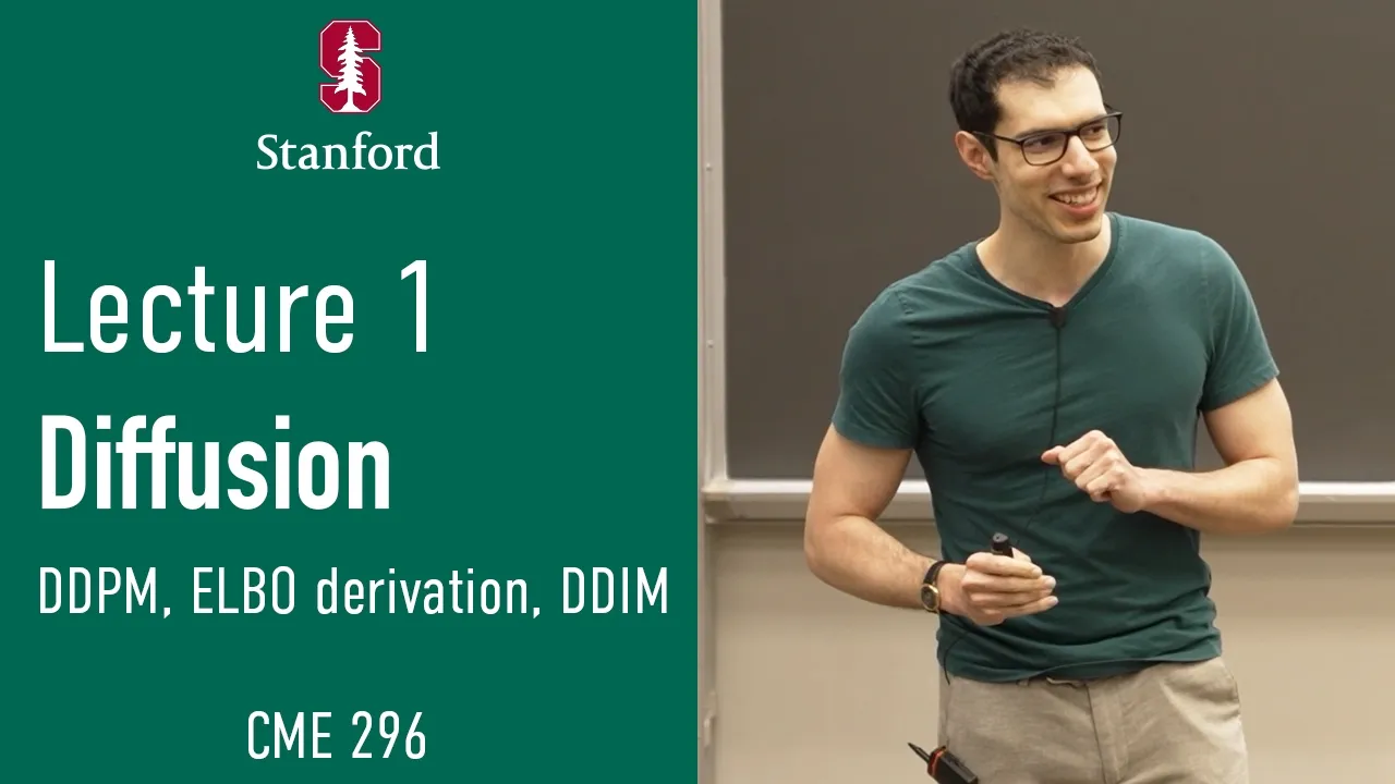
Stanford CME296 Diffusion & Large Vision Models ｜ Spring 2026 ｜ Lecture 1 - Diffusion — Annotated Lecture Notes & Key Takeaways

Course Information

Institution: Stanford

Original Course: Stanford CME296 Diffusion & Large Vision Models ｜ Spring 2026 ｜ Lecture 1 - Diffusion

Instructor Bio: This lecture is co-delivered by **Afshine Amidi** and **Shervine Amidi**, adjunct faculty at Stanford University’s Institute for Computational and Mathematical Engineering (ICME). Afshine Amidi earned his engineering degree from École Centrale Paris and a Master of Science in Operations Research from the Massachusetts Institute of Technology, where he worked under Prof. Dimitris Bertsimas and received the Jean Gaillard Scholarship and MIT Dean’s Fellowship. He has held professional roles at Amazon and McKinsey & Company, leading AI and business strategy initiatives, and co-authors widely adopted technical learning guides on machine learning, algorithms, and transformer models. Shervine Amidi holds B.S. and M.S. degrees in engineering from École Centrale Paris, as well as an M.S. in Computational and Mathematical Engineering from Stanford University. He has conducted computer vision research at the Stanford Vision Lab and the École Centrale Paris Visual Computing Center. Currently a Senior Machine Learning Engineer at Netflix, he previously worked at Google DeepMind on the Gemini team, Google Assistant, and Uber’s data science division. He has served as a teaching assistant for multiple core Stanford CS courses and has been an adjunct lecturer at the university since 2021.

Course Description: As the opening session of CME 296, this lecture establishes the broader context of generative computer vision and motivates the emergence of diffusion probabilistic models as a dominant generative paradigm. It covers the core formulation of Denoising Diffusion Probabilistic Models (DDPM), the formal derivation of the Evidence Lower Bound (ELBO) objective, the standard forward noising and reverse denoising diffusion process, and accelerated sampling techniques enabled by Denoising Diffusion Implicit Models (DDIM).

Lecture 1 of Stanford's CME296 series is where the diffusion​ material actually begins, and Afshin — who runs the session — doesn't pretend otherwise. He opens with a side-by-side: the kind of output he and his twin brother Shervin were getting in 2014, small grayscale things, mostly digits and faces, set against the sharp full-color plates he pulled from ChatGPT the week of the talk. Ten years of progress compressed into one slide. The whole course is aimed at explaining how that jump happened and why the modern approach holds together.
 

Setting the Stage, the Prerequisites, and the Eight-Week Roadmap

 

The two instructors have near-identical résumés, which is a running joke in the first three minutes: engineering school at Centrale Paris in France, then US grad school — MIT for Afshin, Stanford's ICME department for Shervin — then Uber, Google, and now Netflix for both. Their first projects a decade back were computer vision, and that's the stated reason they're teaching it.
 

Course goals are stated as two things: understand the paradigms that let you generate images at all, and understand how the underlying models get trained and evaluated. Nothing about prompt engineering or tool use. This is a mechanics class.
 

Then comes the part I'd want you to read before deciding whether to stay enrolled. Afshin is unusually direct that the prerequisites are real. Linear algebra, with vector-field divergence explicitly on the list (a slightly unusual ask, and a hint about where the later lectures go). Probability: Bayes, conditionals and marginals, expectation, covariance matrices, the Gaussian. Differential equations — he mentions ODEs and SDEs as things you'll end up solving. And general ML literacy: what training and inference are. He softens it by promising the class won't assume mastery, and by saying the emphasis will be intuition rather than exhaustive detail, since papers in this area are wall-to-wall formulas. That's a promise that gets tested later in the same lecture.
 

Logistics, briefly, for whoever's catching up: Fridays 3:30–5:20, two units, letter grade or credit/no-credit. Recordings go up by Saturday evening, so remote attendance is fine. No homework at all. Two pen-and-paper exams, a midterm and a final, ninety minutes each, with the midterm roughly four weeks out. He points at CME295, the LLM-focused sibling course, as a reference for what the exam style looks like, and mentions a sample is linked from the site. Slides post Thursday evenings for annotation, there's a four-page cheat sheet collecting the main formulas and concepts, announcements go to Canvas, discussion to Ed.
 

One detail worth flagging early: he warns that notation in this literature is genuinely inconsistent. The time index runs 0 to 1 in some papers, 0 to T in others, sometimes reversed; the noise variable shows up as ε, z, x₀, x₁ depending on the author. The class commits to using the most common conventions, staying internally consistent, and calling it out when it isn't. Also, papers referenced at the bottom of slides are optional — not examinable.
 

The roadmap is the most useful slide in the first twenty minutes. The framing is a prompt going in ("a teddy bear reading a book") and an image coming out, then a breakdown of the moving pieces:
 

• Lectures 1–3 cover how generation happens at all: diffusion, score matching, flow matching.
• Lecture 4 covers conditioning, plus representing images in a space that "makes sense" — the latent representation.
• Lecture 5 is architecture: U-Nets as the historical default, and the current convergence toward transformers, the diffusion transformer and multimodal variants.
• Lecture 6 is training, post-training, and distillation for when you need the model faster.
• Lecture 7 is evaluation, which he admits is genuinely hard to pin down.

 

Crucially, the first three lectures assume no conditioning input at all. No prompt. The setup is pure unconditional sampling: you have a training distribution and you want new draws from it. That abstraction is what lets Lecture 1 stay focused.
 

Why Every Generator Starts in Static

 

Before any math, Afshin spends real time on a question that sounds obvious and isn't: why does generation begin from noise?
 

He gives three reasons. Noise is trivial to sample — draw from a Gaussian and you're done. Noise carries randomness, so two runs from different starting points land on different images, which is the entire mechanism behind output diversity. And the Gaussian has algebraic properties that collapse a lot of otherwise brutal math.
 

He reaches for a sculpture analogy: a sculptor starts from a block of rock whose shape is arbitrary and differs from block to block, and carves from there. There's a Michelangelo line on the slide to go with it. I like the analogy for the diversity point and I think it's loose on the rest — a sculptor removes material from something that already has structure, while Gaussian noise has none. Don't lean on it too hard.
 

A student pushed back with the obvious alternative: why not a blank canvas? The answer is the cleanest moment in the lecture. If your sampling procedure is deterministic and you always begin at the same point, you always arrive at the same endpoint. The randomness has to enter somewhere, and putting it at the start is the cheapest place to put it. Keep this answer in your pocket — it comes back in the last section, because it's exactly the property that makes DDIM work.
 

Then the ground-clearing. An image is a grid of pixels, each with red, green, and blue values, so you can flatten it into a vector of dimension pixels × 3. Afshin stresses this is not the representation practitioners use and that lecture 4 will replace it. So everything in this lecture is built on a representation you're about to abandon — worth knowing, because it means the math here is foundational rather than final.
 

Next, a Gaussian refresher aimed at people who've only seen the scalar version. Random variables can be vectors; then the mean is a vector and the variance becomes a covariance matrix. Most of the time the class simplifies that covariance to σ² times the identity, which is what "isotropic" means — the spread is identical in every direction, picture a circle rather than an ellipse. And the Gaussian density has a clean closed form, which is the whole reason it keeps showing up.
 

Noise, formally, is ε drawn from a standard normal: zero mean, identity covariance. A question from the room raised whether pixel values are discrete or continuous, since the values run 0–255. The answer: in practice they're rescaled into a float range, so treat them as continuous. Another exchange clarified that the independence assumption applies to the noise, not to real images — noise is drawn independently per coordinate, images obviously aren't.
 

Building the Diffusion Objective, One Trust-Me Step at a Time

 

The anchor is DDPM, described as the first successful application of the diffusion idea to images. The goal for the rest of the session: understand what makes it work and how you get to its loss function.
 

Corrupting on purpose: the forward process, the schedule, and a shortcut

 

The framing is a pair of processes. The forward process, written q, is yours to design. You take a training image and degrade it step by step, x₍ₜ₋₁₎ → xₜ, adding Gaussian noise as you go. The reverse process is what you want to learn — a model with parameters θ that goes from a noisy image to a slightly cleaner one.
 

The update itself is a weighted blend: scale the previous image down, scale some fresh noise up, add them. Written with β as the noise coefficient, then reparameterized with α = 1 − β, it's the familiar square-root form. Two things get asserted here. First, the coefficients are chosen so total variance is preserved from step to step — the "variance preserving" property, whose motivation gets deferred to a later lecture. Second, the β values are not constant. They form a noise schedule, ramping up gradually: a whisper of noise near the clean end, a lot near the noisy end. The stated reason is about what's learnable — small perturbations near the clean image force the model to pick up fine detail; heavy corruption near the noise end leaves only coarse structure to recover.
 

That's a satisfying story, and nothing in the lecture demonstrates it. It's intuition, offered as intuition.
 

The payoff is a shortcut. Because the noise terms are independent Gaussians, and the variance of a sum of independent Gaussians is the sum of the variances, you can collapse the whole chain. Define ᾱ as the running product of the α's, and you can jump from the clean image straight to any timestep t without walking through every intermediate step. Afshin proves this on the blackboard and is candid that the course won't have time for every derivation — slides will carry a footnote naming the trick, and anything not derived in class won't appear on an exam. Useful calibration if you're watching for credit.
 

The quantity nobody can compute, and the bound that replaces it

 

Now the actual objective. The standard move is maximum likelihood: find parameters that make the training data as probable as possible under your model. He notes in passing that everyone works in log space — the log function behaves well, and probabilities between zero and one get numerically fragile when multiplied out.
 

There's a refresher on joint distributions, the chain rule, and marginalization, with a heat map: a joint density over two variables, a conditional as one normalized column, a marginal as the sum down the rows. All of it generalized to T variables, with the compact notation p(x₀:ₜ) for the joint.
 

Then the wall. To get the marginal probability of a clean image under your model, you'd have to integrate over every intermediate state — every possible trajectory from noise to image. There are too many trajectories and the vectors are enormous. The quantity is correct and completely unusable.
 

The escape is the standard one: optimize a lower bound instead. If you push a bound up, you're at least making progress on the thing you care about. That's the ELBO, the evidence lower bound.
 

The derivation here is the most interesting stretch of the lecture. You multiply by q over q — a ratio equal to one, but a deliberate one, because q is the process you defined and therefore know. That converts an intractable integral into an expectation over trajectories sampled from the known forward process. Then Jensen's inequality, since log is concave, moves the log inside the expectation and locks in the bound. The conceptual shift is worth stating plainly: you stop summing over all conceivable paths and start sampling from paths your own noising procedure generates.
 

From there, the bound decomposes. Some terms don't depend on the parameters and get ignored. What survives is a KL divergence between two distributions: q of the less-noisy image given both the noisier one and the clean one, versus the model's p_θ of the less-noisy image given only the noisier one.
 

KL divergence gets its own refresher — a weighted log-ratio, a sum in the discrete case, an integral in the continuous case, equivalently an expectation. Then the key move: showing both sides of that divergence are computable.
 

For q, apply Bayes. The target is proportional to a likelihood times a prior. The forward process is Markovian, so the likelihood reduces to the single-step transition. The denominator doesn't involve the variable you're solving for, so it's just a constant. You're left with a product of two Gaussians, and a product of Gaussians is Gaussian — so q(x₍ₜ₋₁₎ | xₜ, x₀) is an exact normal distribution whose mean depends on the noisy image and the noise that produced it. Afshin calls this "a little bit of cheating," and he's right to flag it: at training time you have the clean image, so this is computable. At inference time you don't, which is precisely the gap the model has to close.
 

For p_θ, we simply choose it to be Gaussian, on the grounds that the true reverse transition is approximately Gaussian. With two Gaussians and both densities in closed form, the KL divergence simplifies dramatically, and what falls out is an L2 distance between the noise the model predicts and the noise you actually added.
 

Two Gaussians and an L2 loss

 

The resulting training objective is startlingly plain. Sample a clean image, sample a timestep, sample noise, build the corrupted image in one shot using the closed form, hand the corrupted image and the timestep to the model, and penalize the squared error between predicted and actual noise.
 

Two details are worth pulling out. The model receives the timestep as an explicit input, not just the image, so it knows how much noise it's looking at and can calibrate. And the "predict the noise" target isn't the only possible parameterization — it's the one that falls out of this particular derivation.
 

There's also a subtlety he admits he'd been hiding. Simplifying the KL divergence actually yields the L2 term times a set of coefficients, which act as per-timestep loss weights. Those weights are a design choice. The DDPM authors experimented with the full weighted version and with setting the weight to one, and found the simple version acceptable. This is one of the few points in the lecture where the instructor openly says: this is a knob, and here's what the original authors did with it.
 

Training is then anticlimactic in the best way: build corrupted images, predict noise, backpropagate. Sampling runs the reverse loop from T down to 0, subtracting the predicted noise and re-adding noise scaled to the standard deviation of the learned distribution at each step, because p_θ is a distribution and sampling from it means drawing from it.
 

DDIM: Turning a Thousand Steps Into Twenty

 

Shervin takes over around (1:29:51) — the auto-caption garbles a name at the handoff, but it's him — and picks up the practical problem the derivation leaves behind.
 

T is large. On the order of a thousand in the original work. Compare that with VAEs or GANs, where generating one image is a single forward pass; if that pass costs a hundred milliseconds, a thousand-step loop costs minutes. Nobody ships that.
 

His first attempt at fixing it is the naive one: write out the recurrence for a subsequence of timesteps, τ, with gaps bigger than one. It doesn't help. You still need one model evaluation per skipped step, so the cost is unchanged.
 

The second attempt is to guess an update formula that links distant steps directly, and check it reduces to the known relation when the gap is one. It does. But quality degrades as the step size grows, and Shervin ties the degradation to the stochasticity injected between steps.
 

So the requirement becomes precise. Find a family of forward processes, indexed by σ, that (a) reproduces the same per-timestep marginals as DDPM, and (b) permits a deterministic generative step. Setting σ to zero gives zero variance, so x₍ₜ₋₁₎ becomes a one-to-one function of xₜ with no noise term. That's DDIM — denoising diffusion implicit models, where "implicit" means the randomness isn't visible between steps; it lives entirely in the initial noise draw. And this is where the earlier blank-canvas question pays off: Shervin points out that if you always started from identical noise, DDIM would produce one image forever, because the initial draw is the only source of variation.
 

The update is built by rearranging the marginal relation to estimate what the clean image probably looks like at the current step, then plugging that estimate back in to construct the previous step. No added noise, by construction.
 

Then the skipping works. You run the same update along a subsequence τ of length S instead of all T steps, giving an effective speed-up of T over S. Typical speed-ups sit between ten and a hundred, with ten to fifty being the practical range, and it's an explicit speed-versus-quality trade. He shows a chart of FID — Fréchet Inception Distance, which he explicitly defers to lecture 7 — and cautions that the absolute numbers mean little and only the relative gaps matter. At roughly a 20× speed-up, quality reportedly stays close to the no-skipping baseline.
 

Where the Argument Felt Thin

 

This is a strong lecture, and I'd still rank it as one where the middle third asks you for a lot of faith.
 

Three trust-me moments stack up in about ten minutes. The ELBO-to-KL decomposition is asserted with "I will need you to trust me that this is equal to this." The mean of the Gaussian posterior is given as a formula with "please trust me." And the assumption that the reverse process is Gaussian is justified by an appeal to the true reverse being approximately Gaussian, with the actual justification dismissed as too far into the weeds. Individually each is fine and standard — every treatment of this material does it, and the time budget is genuinely tight. Stacked, they mean the single most important claim in the lecture, that the intractable objective reduces to noise regression, rests on steps most of us took on credit.
 

Two motivations get deferred outright: why the variance-preserving coefficients have that particular form, and why the increasing schedule helps learning. Both are asserted as things we'll see later. That's an honest thing for an instructor to say, but it means Lecture 1 defines its forward process before justifying it.
 

The DDIM half has a different problem. Shervin says up front that formula density goes up and the goal is intuition. Even so, a student interrupted with "where's the skipping steps here?" — a fair question, because the construction of the deterministic update is presented before it's clear what it buys you. He also declines to show the comparison against samplers that keep the stochasticity, referring to the paper instead, and warns that the FID numbers on screen shouldn't be read as absolutes. So the central empirical claim of the section — determinism beats stochasticity when you skip — is one we're asked to accept secondhand.
 

One more, smaller: the sculpture analogy. The rock a sculptor starts from has grain, faults, and a shape that constrains what can be carved. Gaussian noise has none of that. It works for the diversity argument and I'd retire it after that.
 

If you're reviewing before Lecture 2, the three things I'd actually nail down are the closed-form jump from x₀ to xₜ via ᾱ, the reason multiplying by q over q converts an integral into a samplable expectation, and the exact sense in which DDIM keeps DDPM's marginals while dropping its per-step randomness. Everything else in the session hangs off those.
 

Afshin's closing reassurance is that this is probably the hardest of the eight — which, given that it carries an entire derivation from maximum likelihood to an L2 loss, seems credible.
 

Content Disclaimer:

This article is for general reference only and does not constitute professional R&D guidance, production process advice or quality certification. All material performance data has specific test premises; readers should verify parameters against actual equipment and working conditions.