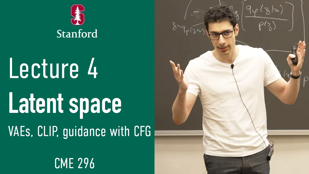
Stanford CME296 Diffusion & Large Vision Models ｜ Lecture 4 - Latent Space & Guidance. — Annotated Lecture Notes & Key Takeaways

Course Information

Institution: Stanford

Original Course: Stanford CME296 Diffusion & Large Vision Models ｜ Spring 2026 ｜ Lecture 4 - Latent Space & Guidance.

Instructor Bio: This lecture is co-delivered by **Afshine Amidi** and **Shervine Amidi**, adjunct faculty at Stanford University’s Institute for Computational and Mathematical Engineering (ICME). Afshine Amidi earned his engineering degree from École Centrale Paris and a Master of Science in Operations Research from the Massachusetts Institute of Technology, where he worked under Prof. Dimitris Bertsimas and received the Jean Gaillard Scholarship and MIT Dean’s Fellowship. He has held professional roles at Amazon and McKinsey & Company, leading AI and business strategy initiatives, and co-authors widely adopted technical learning guides on machine learning, algorithms, and transformer models. Shervine Amidi holds B.S. and M.S. degrees in engineering from École Centrale Paris, as well as an M.S. in Computational and Mathematical Engineering from Stanford University. He has conducted computer vision research at the Stanford Vision Lab and the École Centrale Paris Visual Computing Center. Currently a Senior Machine Learning Engineer at Netflix, he previously worked at Google DeepMind on the Gemini team, Google Assistant, and Uber’s data science division. He has served as a teaching assistant for multiple core Stanford CS courses and has been an adjunct lecturer at the university since 2021.

Course Description: This lecture shifts focus to latent-space generative systems and controllable generation mechanisms. It explains the architecture and training of Variational Autoencoders (VAEs) and how they enable diffusion models to operate in compressed, semantically meaningful latent representation spaces. It also covers vision-language representation learning via contrastive learning frameworks including CLIP and SigLIP, and explains both classifier guidance and classifier-free guidance techniques for enabling precise, controllable text-to-image generation.

The lecture opens on a reassuring note: the speaker tells the room that the first three sessions were the most technically and mathematically punishing stretch of the course, and that what follows will lean on them as building blocks rather than adding more heavy machinery. The specific gap he wants to close is that everything so far has been unconditional generation, and the whole point of a usable image model is that you can point it at something. That turn — from "generate an image" to "generate this image" — is what eventually forces the question of where generation should happen at all, and his answer is the latent space.

Where Lecture 4 Picks Up: Three Lectures of Math, Then a Shift to Conditioning

Before anything new, there's a brisk recap. Lecture one built the DDPM picture: take clean images, corrupt them in discrete steps by mixing them with Gaussian noise under a set of coefficients, and train a network to reverse the damage. The math collapsed into a tidy objective — an L2 loss on the noise that was added — and the denoising rule moved you from step t to step t−1 using a network parameterized on that noise, written epsilon-theta.

Lecture two rederived the same story in continuous time. The increment in x splits into a drift term and a diffusion term, with the noise injection becoming a Wiener increment. A result from stochastic differential equations then says you can write down the reverse process provided you know the score, which is why that whole formulation carries the s-theta parameterization.

Lecture three reframed everything as transporting probability mass from an initial distribution to a target one. Under that view, a noised image is a weighted blend of noise and a sample, and the only thing left to learn is the vector field — the velocity, u-theta.

The recap is efficient, and he uses it to isolate two things the first three lectures quietly assumed rather than argued. First, all of it was written as if there were some obvious way to represent a noised image, some N- or D-dimensional space that x_t just lives in. Nobody said which space. Second, epsilon-theta, s-theta and u-theta are all functions of the noised image and the time step only — no user input anywhere. Today is about both omissions.

The advertised menu has three items: how to represent the noisy images, how to represent the condition you want (a text prompt like a teddy bear reading a book, or a reference image), and how to use that condition to steer sampling. He gives the session its own title — multimodal guided generation.

Worth flagging early, since it shapes how you read the rest: in the transcript I have, only the first item fully lands. The other two are announced, then the speaker hands over to a colleague named Shervin around the 57-minute mark, and the file ends before anything about conditioning is actually delivered.

Why Pixel Space Is the Wrong Place to Diffuse

He starts with the representation anyone would reach for. Images come to us as pixels, each one carrying three intensities for red, green and blue, stacked into a tensor of height, width and three channels. The total dimensionality is three times H times W (7:28).

Then come three objections, and they build rather than sit side by side.

The first is blunt: a 1024 by 1024 image puts you at roughly ten to the sixth dimensions. Every generation paradigm he just spent three lectures deriving scales with the dimension it operates in, and a million is not a friendly number.

The second is redundancy. Look at any small neighborhood of pixels and the values are nearly identical. By his framing that's wasted dimensions — the representation is carrying far more coordinates than the content requires, so it isn't compact.

The third objection is the one that actually does the work, and it's specific to diffusion rather than to compression generally. If you nudge an image slightly in pixel space by adding noise, you don't drift toward a neighboring plausible image; you get something meaningless. He reaches back to the density sketches from earlier lectures: what you want is clusters of likely observations, and what the pixel representation gives you is a spiky landscape where each spike is one valid image and the space between spikes is junk. A generative model that starts from a standard normal and has to walk to a target does not survive that geometry.

From those three complaints he extracts a wish list — tractable dimensionality, compactness, and meaningfulness, where "meaningful" has a concrete operational definition: the valid images should form clusters you could actually aim at.

There's a terminology detour here that I'd have skimmed on the first pass and probably shouldn't have. He defines semantic similarity as agreement in global geometry and overall structure: two pictures of a teddy bear reading a book, not aligned pixel for pixel, still semantically similar. Perceptual similarity is the lower-level notion, about local detail and texture — he shows a second teddy bear, this one with small glasses, and the point is that to a human eye the images read as the same. He stops to ask whether the distinction is clear because he plans to use both terms later.

It's a fair thing to pin down. It's also slightly uneven in payoff: perceptual similarity doesn't reappear until the LPIPS loss roughly thirty-five minutes later, and semantic similarity barely appears at all in the portion of the lecture I have. I suspect it's setup for the guidance half that got handed off.

The Autoencoder, and Why Its Latent Space Still Isn't Good Enough

The first fix is the obvious one. Put the image through an encoder that outputs something of lower dimensionality — big H, big W and three channels go in; little h, little w and some channel count c come out — then run that through a decoder whose job is to hand back the original. That squeezed middle is the bottleneck, and the whole setup is an autoencoder. The spatial compression ratio, big H over little h, is typically around eight (18:01).

He keeps the architecture at a deliberately shallow level, since the next lecture goes deeper. An encoder is mostly convolutions — a filter scanning the image to produce an activation or feature map — plus pooling, which aggregates patches by maximum or average and buys some spatial invariance by coarsening the granularity. The decoder runs the same ideas backwards with upsampling, and training is plain L2 between the input and the reconstruction.

Then he stops and asks the room directly whether this is a good model (21:11), and answers it against the wish list. Tractable dimension: yes. Compact: yes. Meaningful: not necessarily. Nothing in the objective says anything about the shape of the latent space; the model is incentivized to reconstruct and indifferent to how the codes are arranged, so you can still end up with the same spiky scattering. His reason for caring is sharp: every one of the paradigms from lectures one through three starts from a normal distribution, and if the valid points are flung far apart, the sampler has nothing to steer by.

The fix is to constrain the space instead of hoping for one. Instead of mapping an image to a single code, the encoder now emits two things — a mean and a variance — and the code is drawn from the resulting distribution. On top of that, the per-image distribution is pushed to approximate a standard normal, the prior. He's candid that this is unnatural on first encounter and that it confused him when he first saw the model.

On the decoder side the symmetric idea appears and is immediately trimmed: it emits a mean and a variance too, but the variance gets fixed to a constant, because in pixel space a bit of extra noise doesn't change the image much. Sometimes people just take the mean. He calls this a detail, which is fair.

Two questions from the room pull out things the slides don't say. If you want to reconstruct, the code comes from the encoder's distribution; if you want to generate something new, you draw it from the prior. And if the VAE is already generative, why bother with diffusion at all — his answer is that the VAE goes from latent to pixels in a single step, whereas diffusion and flow matching spread the work across many steps and let you spend more compute. He says there are further differences he hopes to reach if time allows.

The derivation, and what "variational" actually buys

The loss for this thing isn't obvious, because distributions are now everywhere, so he derives it. Start from maximum likelihood: find parameters that maximize the probability the model assigns to the data, or more conveniently the log of it. Write p(x) as an integral over all latents of the prior times the decoder's conditional. That integral can't be evaluated — z is still high-dimensional, and you'd need to sweep an enormous number of codes to estimate it.

The move is the same trick as in lecture one. Multiply and divide by the encoder's distribution, which converts the integral into an expectation over just the codes the encoder thinks are plausible for this image. His metaphor: searching every latent is like being dropped in the ocean and told to look through all of it, when only a small subset of codes could have produced this particular image. Take the log, apply Jensen's inequality to pull it inside the expectation, and you have a tractable lower bound.

Splitting that bound with log rules gives two terms. The first is an expected log-likelihood of the image given the code, and because the decoder's output distribution is Gaussian with fixed variance, its log density reduces to a distance between input and reconstruction. That's the reconstruction term. The second is a KL divergence between the encoder's distribution and the prior, which penalizes the codes for wandering away from the standard normal. A coefficient in front of it controls how hard you push: push hard and the latent genuinely looks normal; push too hard and the prior, which knows nothing about the input, takes over and the model stops using the image at all. He names that failure mode — posterior collapse (46:15).

One thing I'd flag as a listener: the reconstruction-to-L2 step is asserted rather than shown. He says outright that it hasn't been derived here and that taking the log of a Gaussian density is what produces it. That's true, and it's a short calculation, but it's the one place where a student trying to reproduce the derivation from the slides alone would get stuck. Also note that the checklist quietly grew a fourth criterion — truthfulness — only after the model cleared the first three. It's a real requirement, but it wasn't on the original wish list.

Blurry Reconstructions, and Two Patches for Them

Truthfulness is where the VAE fails, and the failure has a specific shape: reconstructions come out blurry. The mechanism is the pixelwise L2. If the output is off by a few pixels from the input, the penalty is large, so the model hedges by producing values close to an average of what it thinks the answer might be. Averaging across plausible outputs is what blur looks like. He notes the plain autoencoder has the same defect, but the VAE makes it worse, precisely because an image no longer maps to one point but to a whole distribution of codes, which injects additional uncertainty into what the decoder should commit to.

This matters for the course's actual aim. If diffusion is going to run inside a latent space and the decoder is the last thing standing between a clean latent and a finished picture, a blurry decoder undoes the whole exercise.

The first patch replaces the comparison rather than the model. Instead of scoring input against output pixel by pixel, push both through a convolutional network and compare their feature maps. Feature maps are spatially invariant in a way raw pixels aren't — shift an image slightly and the maps barely move. The named instance is LPIPS, learned perceptual image patch similarity (52:27), a weighted sum of feature-map differences with weights tuned to match human judgments of similarity. He's refreshingly dismissive of the formula itself: what matters is that you're comparing feature maps, not pixels.

His caveat is the useful part. Crank the perceptual weight too high and you don't get sharper images, you get checkerboard artifacts — grid-like patterns baked into the output (54:03). So the weight has a sweet spot, and neither extreme is free.

The second patch changes the training game entirely. Add a discriminator whose job is to tell decoder output from real images; a blurry reconstruction gets flagged as fake, which penalizes the decoder for producing one. The decoder then tries to fool the discriminator, the discriminator tries not to be fooled, and the decoder is pushed toward outputs that look real. He's explicit that there's no time for GAN details and that the slide is meant to carry it.

That's the part I'd most want expanded if there were another twenty minutes. Three loss terms now have to be balanced — reconstruction, perceptual, adversarial — and no guidance is given on how to set those weights or what happens when they fight. For a lecture that otherwise does real derivations, this section is unusually gestural.

Stitching the VAE Together With Diffusion and Flow Matching

The payoff arrives quickly at the end. Everything above exists so the generative model can run in the learned latent space instead of pixel space, which is computationally cheaper and scales.

Training happens in two stages. First the VAE is trained as described. Then the generation model is trained inside its latent space: take an image, encode it to a mean and a standard deviation, sample a code, treat that as the clean endpoint, form a noised version as a weighted combination with noise, and fit the velocity with an L2 objective — he uses flow matching as the illustration.

Inference inverts it. Sample noise in the latent space, integrate the learned velocity numerically to reach a clean latent, then hand that to the VAE decoder to get pixels. He's mid-demonstration of what that looks like when the transcript stops.

Two loose ends are worth naming, because they're the kind of thing that quietly becomes an exam question. The deferred comparison between VAEs and diffusion/flow matching never gets resolved here — he says he hopes to get to it if there's time, and there isn't. And the two menu items about conditions — how to turn a text prompt or a reference image into something a sampler can consume, and how to use it to steer the trajectory — are announced in the first two minutes and then handed off at 57:04. The file I have ends at 59:58, mid-sentence, before any of it lands.

So the honest summary of this session is that it's a complete, well-paced treatment of one half of its title. The argument for leaving pixel space is genuinely well built: three concrete complaints, a wish list derived from them, a model that satisfies two of the three, a loss derived from first principles that buys the third, and then an honest accounting of what the fix costs you in fidelity. The latent space you end up with is tractable, compact, structured and, until you bolt on perceptual and adversarial terms, slightly blurry. What I can't tell you from this file is how a prompt gets attached to any of it — that's the half of the lecture I'd go find before the next one.