Stanford CS336 Language Modeling from Scratch | Lecture 2: PyTorch and einops — Annotated Lecture Notes & Key Takeaways

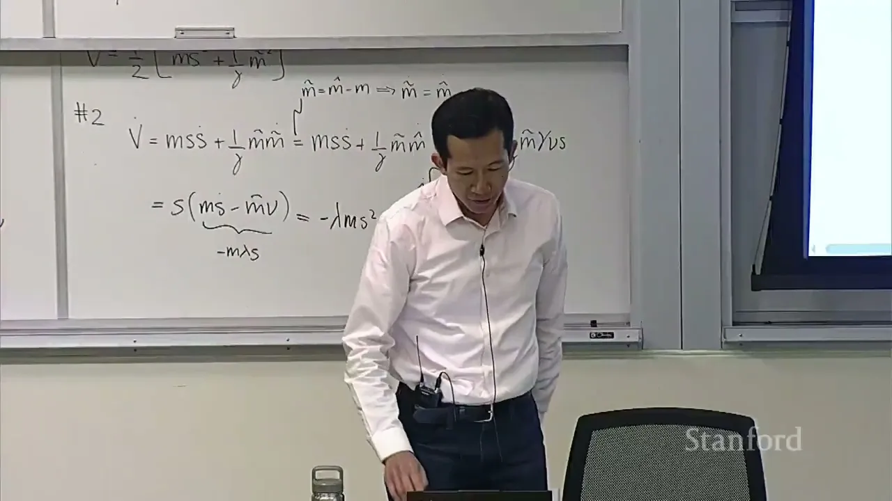
Course Information

Institution: Stanford

Original Course: Stanford CS336 Language Modeling from Scratch | Spring 2026 | Lecture 2: PyTorch and einops

Instructor Bio: This lecture is delivered by **Percy Liang**, Associate Professor of Computer Science at Stanford University and core faculty of the Stanford Institute for Human-Centered Artificial Intelligence (HAI). Percy Liang leads the Stanford Natural Language Processing Group, with research spanning the theoretical foundations and practical systems of language modeling, machine learning alignment, compositional semantics, and NLP evaluation. He received his PhD in Computer Science from the University of California, Berkeley and his BA in Mathematics from Harvard University. His work has been recognized with the NSF CAREER Award, Google Faculty Research Award, and multiple best paper awards at top-tier machine learning and NLP conferences. He is also widely known for creating influential benchmarks and open-source frameworks for language model research and assessment.

Course Description: This lecture covers the practical software engineering foundations for implementing language models using PyTorch, with a special focus on the einops library for clean, readable tensor operations. It reviews core PyTorch concepts relevant to deep learning systems, explains how einops simplifies common tensor manipulation patterns — including reshaping, permutation, and reduction — that are ubiquitous in transformer architectures. The session walks through hands-on implementation best practices for building modular, maintainable, and performant model components, bridging theoretical architecture design with real code implementation.

He opens with a weather joke — "I hope everyone is staying dry," followed immediately by "I'm not" — and then shares something he's clearly pleased about. A scaling-law experiment he'd been running finished, and the loss landed within 0.05 of what the fitted curve predicted. He'd been fitting what he calls iso-FLOPs curves: run a family of small models, find the compute-optimal point on each curve, extrapolate, then actually run the big one and check. It matched. Extrapolating further gets you to a GPT-5-level loss, with the usual caveat that the extrapolation is only as good as the scaling law underneath it.
 

That anecdote sets the mood for the whole session. This is a lecture about counting things before you try to optimize them, and the payoff is that the counting sometimes works.
 

The stated topic is resource accounting​ — the systems side of the course. The governing goal is to train the best possible model under a fixed budget of compute and memory; data, he says, won't be the binding constraint for this class. Before you can improve computational efficiency, you need to be able to describe the efficiency of a given computation, and that means knowing its compute and memory characteristics.
 

Two warm-up questions do most of the framing work. First: how long to train a 70-billion-parameter model on 15 trillion tokens across 1024 H100s? His answer plods through the arithmetic — FLOPs are roughly six times parameters times tokens, look up the H100's throughput, assume a model FLOPs utilization of 0.5, convert to days — and lands at 143 (2:46). Second: what's the largest model you can fit on eight H100s with AdamW? Eighty gigabytes of HBM per card, twelve bytes per parameter once you add up the pieces, and you get something in the neighborhood of 53 billion (3:23). He flags immediately that this ignores activations, which depend on batch size and sequence length, and says outright that the point is not precision but getting "the rough shape of things."
 

Then the meta-framework carried over from lecture one: mechanics (how PyTorch and tensors actually work — "no magic here"), mindset (get into the habit of asking what a line of code costs), and intuitions (where the resources go). No machine-learning magic in this one; that's Tatsu's job next week, on architectures.
 

Tensors and Precision in PyTorch: How Few Bits Will You Accept?

 

Everything is a tensor. Parameters, gradients, optimizer states, data, activations — all of it. He points at DeepSeek 3.2 as an example and notes that a model is really just a pile of tensors, each with a shape and a precision (5:06). Memory math is as boring as it sounds: number of elements times bytes per element.
 

The precision tour is where the section gets interesting. A standard float is float32 — one sign bit, eight bits of exponent (which buys dynamic range), the remainder as mantissa (which buys resolution). The term "single precision" is a fossil from scientific computing, where float32 was the floor you'd expect by default and float64 was the upgrade. Deep learning runs the other direction, because 32 bits is more than these computations need.
 

A four-by-eight matrix of float32 is 128 bytes, which sounds like nothing until he mentions that a single feed-forward matrix in GPT-3 is around 2.3 gigabytes (7:54). Cutting precision helps twice over: fewer bytes to store, and operations on narrower types run faster — roughly twice as fast, though he hedges that with "not always." The second-order effect, that saving memory can also save time, is the one he promises will make sense later.
 

The naive move is to halve the bits and call it float16. That gets you five exponent bits, and five is not enough: try to build a tensor of 1e-8 and you get zero. People did train in FP16 back in the day and it was miserable — underflow, overflow, NaNs.
 

BFloat16, developed in 2018, is the fix, and the trick is almost insultingly simple (9:55). Keep sixteen bits, but move bits out of the mantissa and into the exponent. You end up with the same dynamic range as float32 and worse resolution. There's no free lunch, but in deep learning the trade is usually worth taking, because what you desperately want is to avoid over- and underflow, and the computations are noisy enough that fine resolution doesn't buy much.
 

For training, then: float32 is fine for small models and costs four bytes per parameter; float16 is too fragile; BF16 is the sweet spot, though he adds that even BF16 can be risky. The common practice is mixed precision — BF16 for parameters, activations, and gradients, FP32 for optimizer states — which PyTorch's AMP library will do for you by casting to BF16 where it judges it safe (matrix multiplications: yes; exponentials: no) (11:53).
 

If you want to go further, FP8 arrived about four years ago and comes in two flavors, trading dynamic range against resolution; Nvidia's Transformer Engine supports it. And then there's FP4. NVFP4, from last year, gives you four bits per value, which he illustrates by saying he can write every representable value on one line, somewhere between roughly −6 and 6. That's not enough on its own, so there's a cheat: values live in blocks, and each block carries its own scale factor. A single value therefore gets more than four bits of effective dynamic range — you just can't have one element enormous while its neighbor is microscopic. A model called NeMo-3 Super was reportedly trained in FP4 this year. Much of this lives inside Nvidia's stack rather than in code you write yourself; you don't casually declare an FP4 tensor.
 

Two student questions close the digression. One asks for clarification on block scaling, and the answer is essentially that the scale gives you range at the block level while the four bits give you resolution within it. The other asks why not go all the way to one bit. The distinction he draws is between training and inference: quantizing a finished model down to one or two bits is hard but well-trodden, whereas training a one-bit language model is something he doesn't think anyone has done credibly (16:47).
 

Last thing in this section, and it's the kind of thing that wrecks beginners: tensors are created on CPU, and you have to move them to the GPU yourself. He ran his slides on a laptop without a GPU, so some code gets shown rather than executed.
 

einops and einsum: Naming Dimensions Instead of Counting Them

 

About two-thirds of the room had used einsum before (18:13). The pitch for it is aimed squarely at the rest of us: code full of transpose(-2, -1) is easy to get wrong and painful to read, because you have to reconstruct in your head what the negative indices refer to. Names beat positions.
 

Think of einsum as generalized matrix multiplication with bookkeeping attached. A three-by-four matrix times a four-by-three matrix is clear enough on its own, but the einsum version names the dimensions — call the first seq1 and hidden, the second hidden and seq2 — and declares the output indexed by seq1 and seq2. Any index that shows up on the inputs but not on the output gets summed away. The operational reading is: walk over every combination of the named indices, pull the corresponding entries out of the inputs, multiply, accumulate into the output.
 

The batched case is where it starts paying for itself. Given two tensors of shape 2×3×4, the old style has you transposing the trailing dimensions and relying on matmul's implicit broadcasting of leading dims. In einops you just write batch, seq1, hidden against batch, hidden, seq2, and out comes batch, seq1, seq2. No transpose appears anywhere. He's explicit that this is the whole appeal: he always loses track of transposes, and naming the dimensions makes the transpose disappear into the notation.
 

Then there's the ellipsis. If you have a pile of leading dimensions — batch, sequence, heads — you can write ... and stop enumerating them, which also means the code keeps working when the shape changes.
 

Two more primitives get a quick pass. reduce generalizes sum, mean, max, and min over named dimensions: name the dims you're keeping, omit the one you're collapsing, pick your aggregation. A student asked whether it's faster; the answer is no, it's sugar over the same primitives. rearrange splits and merges dimensions — the example is a 3×8 matrix where that 8 is really 2×4, so you declare the eight as heads × hidden1, pin heads to two, do your multiplication against a 4×4 weight, then fold it back. There's a follow-up question about ordering when you collapse two dimensions into one (row-major or column-major?), and the answer is that the order you write in the pattern is the order you get.
 

His closing argument for the whole library is honest rather than triumphant: it takes a while to get used to, but once it clicks, transposes and reductions stop being things you think about.
 

FLOPs, MFU, and the Roofline: Why Half the Machine Sits Idle

 

A flop is one floating-point operation, treated as a plain add or multiply, and everything else the silicon can do gets waved away as not the bread and butter.
 

Then a terminological pet peeve worth internalizing (28:17). Lowercase "flops" is a count — the total amount of computation, as in GPT-3's enormous FLOP budget. Uppercase "FLOPS" is a rate — operations per second, a property of hardware, as in the H100's roughly 989 teraflops. He insists on writing /s to keep them apart. Two things follow. Spec sheets list about 1979 teraflops for BF16, but buried in the fine print is the phrase "with sparsity"; for dense work you halve it (29:37). And the practical intuition he wants you to carry is the arithmetic itself: eight H100s for a week is a certain number of FLOPs, this model needs that many, divide. Napkin math, nothing more.
 

Counting the cost of a matmul is where the machinery starts. Data X of shape B×D against weights W of shape D×K runs about 2·B·D·K operations — one multiply and one add per triple, with a −1 that everybody drops. Element-wise operations cost about the size of the tensor. And no other operation you'll meet is as expensive as a matmul once the matrices are big enough, so matmuls are what you count. There's a caveat attached: memory.
 

Someone asked about sub-cubic matrix multiplication algorithms, and the answer is that the optimizations that matter in practice come from co-designing with the system, not from better asymptotics. Another asked whether addition is cheaper than multiplication; on the hardware, no.
 

The useful reframing is that B is your number of tokens and D·K is your number of parameters, which makes the forward pass about two times tokens times parameters. That shape survives the jump to transformers.
 

Then the gap between theory and reality. To time something on a GPU you need CUDA synchronization before and after the operation, because the calls are non-blocking and will otherwise return instantly and make your benchmark look spectacular and meaningless. Do it several times and average. Divide the FLOPs you counted by the wall-clock time and you get achieved FLOPS; compare that against the promised number and you have model FLOPs utilization. Half is something to be happy about for a modern model (37:54). A bare matmul might touch 0.8. If you're sitting at 0.1, something is wrong. A student pushed on what "promised" means, and the answer is worth remembering: it's the spec-sheet figure already halved for sparsity, so the 0.5 stacks on top of that. You're getting roughly a quarter of the headline number.
 

Why only half? Because FLOPs aren't the only thing that costs time, and this is the core of the lecture (40:36).
 

His mental picture of the hardware is deliberately crude: a big pool of high-bandwidth memory, and the compute cores off to the side. To compute anything you have to move tensors from memory into the cores and move results back. The H100 moves about 3.3 terabytes per second (41:52). So runtime depends on two rates, not one, and the standard simplifying assumption is that data movement and computation overlap, making total time approximately the max of the two rather than the sum. Not true in practice, but good enough.
 

Take ReLU over a million-element BF16 vector. You read 2N bytes, write 2N bytes, and perform about N comparisons. Communication time comes out near a microsecond, compute time near a nanosecond. Overwhelmingly, you're waiting on bytes. Memory-bound.
 

Now define two intensities. The accelerator's is its FLOPS rate divided by its bandwidth — for an H100 that's about 295 (46:26), so call it 300: roughly three hundred operations per byte delivered. An algorithm's intensity is its own FLOPs divided by its own bytes moved. If the algorithm's intensity is below the machine's, you're memory-bound; above it, you're compute-bound. Same comparison as before, just rearranged.
 

ReLU's intensity is about 0.25, which he says should read to you as catastrophically low. GELU does roughly twenty operations per element instead of one, so its intensity climbs to around five — still nowhere near 295, and therefore still memory-bound. The consequence is the memorable one: as far as wall-clock goes, ReLU and GELU cost about the same, because neither one is where the time is going.
 

Dot products are worse than you'd hope: read two vectors, write a scalar, intensity around 0.5. Matrix-vector products barely improve, because you ship an entire N² matrix to do N² work. Then matrix multiplication flips everything. Ship two N×N matrices and write one back — order N² bytes — while doing N³ work. In his example the intensity comes out near 340 (51:52), and the general rule is roughly N over three: the bigger the matrices, the better it gets.
 

That single fact explains a lot of received wisdom. Big batch sizes and big matrices aren't an aesthetic preference; below the machine's intensity threshold, shrinking your problem doesn't speed anything up, and only once you cross it do you actually saturate the hardware. Transformers, being mostly large matmuls with odds and ends sprinkled between them, land on the good side of that line, and he says that's not an accident. Decoding at inference time is the mirror image: you generate one token at a time, which turns your matmuls into matvecs, which puts you back on the memory-bound side. Training gets to chew through the whole sequence at once.
 

The visualization is a roofline plot (54:52): arithmetic intensity along the x-axis, realized FLOPS on the y-axis, one curve per accelerator. Low-intensity operations sit on the rising slope where bandwidth sets the ceiling; push intensity far enough right and you hit the flat top, where peak FLOPS caps you and nothing helps.
 

The sharpest moment in the room came when a student pointed out the apparent contradiction: if most of these computations are memory-bound, why are accelerators built with so much compute relative to bandwidth? MFU of 50 percent, maybe 70 or 80 if you're excellent — aren't the cores just idling? He defers it to the GPU lectures and jokes that anyone with an answer should tell Jensen. I wrote that one down as the most interesting question asked all hour.
 

Backprop, Optimizer States, and Trading Compute for Memory

 

The running example is a plain deep network: B×D input, L layers of D×D matrices, each producing pre-activations followed by an element-wise nonlinearity. Parameters are D²·L.
 

Gradient mechanics get one quick demo with a toy regression — a three-element input, a weight vector of ones, an MSE loss — where calling backward populates a .grad field on each tensor in the graph, some set and some not. Basic PyTorch, by his own description.
 

The question that matters is what backward costs. Zoom into one layer, H1 times W2 giving H2. Forward is one matmul. Backward needs two gradients: one with respect to the input, and one with respect to the weights. Both turn out to be matmuls of the same size, so the backward pass costs twice the forward pass (1:05:08). Roll that up over the whole network and you get 2ND forward, 4ND backward, 6ND total — which is where the ubiquitous six-times-parameters-times-tokens formula actually comes from (1:06:12). He notes it's a decent approximation for transformers too, provided the context isn't long; long contexts add a squared term that this accounting misses.
 

On optimization, he deliberately picks Adagrad over Adam, calling it a 2011 ancestor sitting between plain SGD and Adam — momentum tracks first moments, Adagrad tracks squared gradients, Adam does both. Optimizer internals aren't the point here; memory is. The optimizer keeps per-parameter state: Adagrad a single accumulator, Adam two, and because those accumulators are kept in FP32 for stability, that's four bytes per parameter for Adagrad and eight for Adam (1:10:55). He notes that people have tried BF16 states and it goes badly, since you're squaring and averaging over thousands of steps.
 

That's the origin of the 2+2+4+4 from the opening: parameters, gradients, and two FP32 optimizer states. Optimizer memory rarely limits speed, since it isn't what's being hauled into the cores for matmuls, but it's a large, fixed claim on HBM and it's what stops you from fitting a bigger model. He also catches a typo on his own slide mid-explanation.
 

The closing topic is how to buy memory back, and there are two standard tools. Gradient accumulation exists because large batches help stability up to a critical batch size, but activation memory scales with batch (1:12:29). So you split the batch into micro-batches, accumulate gradients without zeroing, and only step and reset every few micro-batches. Activation checkpointing — also called gradient checkpointing or rematerialization — attacks the other side: training stores activations for every layer, whereas inference needs gradients for none, so you store activations for only some layers and recompute the rest during backward (1:13:21). In PyTorch it's roughly a matter of wrapping a block in a checkpoint utility. Applied to a linear-then-ReLU block, skipping the pre-activation tensor saves about half. Store nothing at all and you recompute from scratch for every layer, which costs you L². The balanced choice is to checkpoint at about √L layers, which puts both memory and recomputation overhead at √L (1:16:03). The general principle is one worth stealing: when memory is tight, recompute.
 

His own summary is short enough to repeat in spirit — everything is tensors, einops is a way of thinking, 6ND is now demystified, intensity and rooflines tell you which wall you've hit, matmuls are compute-bound and nearly everything else is memory-bound, and the two memory tricks buy you the headroom to run bigger batches. Next week is architectures.
 

Where the Argument Felt Thinnest

 

Most of this lecture is strong, and the roofline section in particular is the kind of thing that permanently changes how you read a profiler. But a few things didn't fully land for me.
 

The 143-day headline at the top depends on an MFU of 0.5 that isn't justified until forty minutes later. Watching linearly, the first number is an assertion you have to take on faith, and only the roofline discussion retroactively earns it. The 53-billion-parameter figure has a related problem: it excludes activations entirely, and he says so, but for any realistic batch and sequence length that omission is large enough to make the number more of an upper bound than an estimate.
 

The "time is the max of communication and computation" assumption is doing quiet work throughout. He admits overlap isn't perfect, but every intensity threshold downstream inherits the simplification, so the 295 figure is a cleaner boundary in the slides than it is in a real kernel.
 

The accounting for ReLU also feels slightly loose. Counting a compare-against-zero as one flop is fine for the argument being made — the conclusion is robust, since the gap between 0.25 and 295 is enormous — but the units aren't quite the same units used for matmuls.
 

The genuinely unanswered question is the student's: if nearly everything is memory-bound, why keep scaling compute faster than bandwidth? It got a laugh and a deferral. Maybe the GPU lectures answer it, but on the evidence of this session it's the most load-bearing thing left on the table.
 

Finally, a practical note about the medium rather than the content: this is a slide-driven lecture, and several explanations — the FP4 block scaling, the rearrange example, the roofline plot — are hard to reconstruct from audio alone. He skips a worked example at one point, notices his own outputs are stale at another, and can't execute some code because he's on a laptop without a GPU. If you're reading notes instead of watching, budget extra time for those three spots.
 

Content Disclaimer:

This article is for general reference only and does not constitute professional R&D guidance, production process advice or quality certification. All material performance data has specific test premises; readers should verify parameters against actual equipment and working conditions.