Stanford CS336 Language Modeling from Scratch ｜ Lecture 10： Inference — Annotated Lecture Notes & Key Takeaways

Course Information

Institution: Stanford

Original Course: Stanford CS336 Language Modeling from Scratch ｜ Spring 2026 ｜ Lecture 10： Inference

Instructor Bio: This lecture is delivered by **Percy Liang**, Associate Professor of Computer Science at Stanford University and core faculty of the Stanford Institute for Human-Centered Artificial Intelligence (HAI). Percy Liang leads the Stanford Natural Language Processing Group, with research spanning the theoretical foundations and practical systems of language modeling, machine learning alignment, compositional semantics, and NLP evaluation. He received his PhD in Computer Science from the University of California, Berkeley and his BA in Mathematics from Harvard University. His work has been recognized with the NSF CAREER Award, Google Faculty Research Award, and multiple best paper awards at top-tier machine learning and NLP conferences. He is also widely known for creating influential benchmarks and open-source frameworks for language model research and assessment.

Course Description: This lecture focuses on language model inference, covering the algorithms and system optimizations that enable efficient, low-latency model serving. It covers core autoregressive decoding strategies including greedy search, beam search, and stochastic sampling methods, then dives into key inference optimizations such as KV caching, weight quantization, speculative decoding, and dynamic batching. The session analyzes the core tradeoffs between throughput, latency, and memory usage, and discusses best practices for different deployment scenarios from edge devices to cloud-scale serving systems.

If you only watch one hour of CS336 this quarter and you don't plan to become a pretraining person, this is probably the hour to watch. Lecture 10 steps away from scaling laws — Tatsu covered those the week before — and asks a deceptively small question: you've trained a model, someone hands you a prompt, now what? That whole business of turning a prompt into a response, as accurately and as quickly as you can, is inference, and the lecturer's opening argument is that it now matters more than the training run that produced the model in the first place.
 

These notes follow the order of the talk. Where I got lost, I say so.
 

Why Inference Deserves Its Own Lecture

 

The pitch is straightforward but lands hard. Inference shows up everywhere the model is actually used: chat assistants, code completion, agents, batch data processing, any evaluation that requires generation rather than just scoring. It even shows up inside training, because reinforcement learning needs rollouts, and rollouts are just inference with extra steps attached.
 

The cost argument is the one I'd remember. Training is a one-time expense — enormous, but you pay it once. Inference is a repeated expense you incur every day. The number he puts on the board: OpenAI is estimated to produce something like 8.6 trillion tokens a day. For scale, a model in the GPT-4 class was trained on roughly 32 trillion tokens, which means that in under four days of serving, the token volume — and therefore the compute — exceeds an entire pretraining run.
 

Then he sharpens it. The move to agents changed the shape of the problem. In the chatbot era, the bottleneck was the human: people read at a fixed speed, so once generation outpaces reading, extra speed buys you nothing. In an agentic loop, the model thinks, reasons, calls tools, introspects, and only eventually produces something a person reads. Most of the tokens are not for reading at all. Which means generated tokens are better understood as compute spent on a problem, and there's no natural ceiling on how much is worth spending. Squeezing more out of inference has no saturation point the way chatbot latency did.
 

He closes the motivating section with a quick tour of who's doing this work. Closed API providers obviously. A crowd of providers serving open-weight models. And in open source, four packages worth knowing by name: vLLM as the default choice, SGLang as the one tuned for agentic workloads but not yet as widely adopted, NVIDIA's TensorRT as very fast but narrower in scope, and llama.cpp if you want to run on CPU.
 

That sets up the real question: what does fast even mean? He gives three metrics, and the rest of the hour is essentially about how they pull against each other.
 

• Time to first token: how long the user stares at nothing before output starts streaming. This is the latency that hurts most in interactive products.
• Latency: from one user's perspective, how fast tokens arrive for their query. Once tokens start flowing, this can be slower, because the user is reading anyway.
• Throughput: tokens per second across many queries. This is what you care about when you have a pile of documents to process and you just want the job finished.

 

Latency and throughput look like two views of the same thing, and he says up front that most interventions improve both — but then warns there's a real trade-off coming, and spends the back half of the lecture showing where it bites.
 

Counting FLOPs and Bytes: The Arithmetic Intensity Argument

 

This is the intellectual core of the lecture, and it's where I'd tell you to slow down.
 

The claim he wants you to carry out of the room: in training you see every token at once, so the sequence is just another tensor dimension you parallelize over. In inference you don't get that. Generation is autoregressive, one token at a time, and you cannot parallelize across the sequence. Everything distinctive about inference as a systems problem follows from that one asymmetry.
 

Before the argument, a notation detour. He sets up a tensor-diagram convention that he says he finds the crispest available definition of a transformer, because it forces you to state shapes and dependencies instead of hand-waving. Contracting dimensions (present in both operands, absent from the result) are red; dimensions that survive are black; and there's a third category in blue — batch dimensions, present in both operands and kept in the result, neither contracted nor reduced. He flags the blue dimension early and pointedly: remember this one, it's why attention is a bottleneck. The payoff arrives twenty minutes later.
 

Symbols worth writing down: B for batch and number of sequences, T for sequence position, D for model dimension, H for head dimension, N for number of query heads, K for the number of key/value groups, G for query heads per group. F is the MLP width, always taken as 4D. And S versus T both denote sequence-ish quantities — S is how many tokens you're conditioning on, T is how many you're producing logits for. In training S equals T. In inference T equals 1.
 

There's a nice human moment around (19:30) where a student catches an inconsistency in the GQA part of the diagram — that K should be the number of groups and G the heads per group, not the other way around. The lecturer works through it aloud, says "I think you're right," and promises to fix the slides later. If you're reading along with the posted deck, be aware that this labeling may still be wrong.
 

Then the arithmetic intensity review, which was covered back in lecture two. Intensity is FLOPs divided by bytes moved. You compare it against the accelerator's intensity — peak FLOPs per second divided by memory bandwidth, both from the spec sheet. If your computation's intensity exceeds the hardware's, you're compute-bound and the chip is busy doing useful work. If it's lower, you're memory-bound and the chip is idle waiting on data. For a plain matmul on an H100, he works out that you're compute-bound once batch size exceeds about 295.
 

The pathological case is batch size 1, where intensity collapses to 1. You read the whole weight matrix and get to use it exactly once. His comment: you don't get nice fat matrices in inference, you get very thin ones.
 

Now apply that lens to a transformer, counting only the matmuls since everything else is cheap or fusable.
 

MLP layers.​ Intensity comes out around B times T, which is the same story as a plain matmul — an MLP is a big matmul wearing a hat. The batch and sequence dimensions don't interact; each position is independent. At prefill, with large batches and long prompts, you're fine. At generation, T is 1, so intensity collapses to just B. And B during generation means the number of concurrent requests. In a batch job you control that. In a chatbot you don't — it's however many users showed up, which is unpredictable and drifts over the day.
 

Attention.​ Here the intensity works out to S times T over S plus T. At prefill, where T equals S, that's roughly S over 2 — long sequences keep you healthy, though notably the batch dimension doesn't help you at all. At generation, T is 1 and you get S over S plus 1, which is less than 1. Call it 1. Against a hardware target near 300.
 

That's the bottleneck, and he spends real time on why, which I appreciated. In an MLP, every sequence in your batch hits the same weights. Load them once, reuse them across the whole batch, and bigger B genuinely amortizes the cost. In attention, every sequence has its own KV cache, so the memory traffic scales with B. Raising the batch size just means doing more independent matmuls rather than getting more use out of bytes you already paid for. Economically it's closer to running a stack of dot products, which have terrible intensity. And that's exactly the blue batch dimension he flagged at the start, sitting in both operands and refusing to be contracted away.
 

The one-line version he gives: prefill is compute-bound, generation is memory-bound. He adds, with some satisfaction, that now whenever you hear someone say inference is memory-bound, you know why.
 

Latency, Throughput, and the Bus That Never Leaves on Time

 

Once you accept that generation is memory-bound, estimating speed gets much simpler. If you overlap communication and computation, the time is basically the bytes you have to move divided by bandwidth. He calls this simultaneously convenient and annoying — convenient because the model is easy, annoying because your very expensive accelerators are sitting there doing nothing.
 

The worked example is Llama 2 13B on a single H100. He builds up the memory picture in two parts. Parameters: count up the embeddings, the MLP weights, the query/key/value projections, and at BF16 (two bytes per parameter) 13 billion parameters costs about 26 GB. KV cache: for each sequence, it's the number of tokens times the number of KV heads times head dimension times layer count, doubled for keys and values and doubled again for BF16. Add the parameter block to B copies of the per-sequence cache and that's your footprint.
 

At batch size 1 the numbers come out around 8 milliseconds per token, which is about 124 tokens per second — and you can sanity-check that in your head, since 26 GB of weights streaming across H100 bandwidth really is roughly 8 ms.
 

Now turn the batch knob. Latency grows, because there's simply more KV cache to shuffle back and forth. Throughput also grows, because the 26 GB of weights gets amortized across more sequences at once. But throughput doesn't grow without limit — it asymptotes, and long before it gets there you run out of memory. With plain multi-head attention, a batch of 256 doesn't fit on an H100 at all. A B200 pushes the wall outward but doesn't remove it.
 

The analogy he uses is public transit, and it's the one that made the trade-off click for me. A bus has mediocre latency — you wait — but excellent throughput, because it moves everyone at once. And because requests are batched, your individual query waits for the slowest one in the batch.
 

So the design rule is a genuine fork, not a dial:

• Small batches buy you better latency and worse throughput.
• Large batches buy you better throughput and worse latency.
• Anything that reduces memory, by contrast, improves both at once. Only the batch axis is the site of tension.

 

Time to first token slots in cleanly: TTFT is essentially the time to run prefill, because you can't emit anything until prefill is done. So faster TTFT wants smaller batches, while better throughput wants larger ones.
 

He explicitly skips parallelism, mentioning only that you can shard across devices and that the scaling book's inference chapter covers it. The trivial case: run M independent copies of the model, latency is unchanged, throughput goes up by M.
 

Shrinking the KV Cache: GQA, MLA, CLA, and Windows

 

The second half is a tour of techniques, unified by one thesis. Memory is the bottleneck, the KV cache is a large and growing share of that memory — at big batch sizes it can exceed the parameters themselves — so shrink the cache, and both latency and throughput improve. The constraint is that you must not wreck accuracy doing it.
 

Grouped-query attention

 

The most obvious lever, and one the course covered earlier. Standard multi-head attention gives every token its own key and value per head. The extreme opposite, multi-query attention with a single KV head, he dismisses flatly as too bad to be worth using. GQA lives in between: keep all the queries, reduce the number of key/value groups. The cache shrinks by a factor of N over K.
 

The 2023 GQA paper's time-per-sample curves show full attention expensive on one end, K equals 1 fast but damaged, and K around 8 still in the good zone before the curve turns upward. Applied to the Llama example with a one-to-five sparsity ratio, memory drops and both latency and throughput improve. And there's a second-order effect worth noticing: the freed memory let him push batch size to 256, which had previously failed to fit. Latency got a bit worse from the larger batch, throughput improved proportionally. His point is that you tune these jointly — one change moves the feasible set for another.
 

Then the caveat, and it's the most intellectually honest moment in the lecture. Whenever you make a lossy change you must check accuracy, and the GQA paper's evals look fine. But he immediately notes that DeepSeek's later paper shows GQA genuinely hurts. His guidance: treat every result that isn't pure math with suspicion. Coming from the person teaching the class, that's worth internalizing.
 

Multi-latent attention

 

DeepSeek's alternative attacks the same target from a different angle. Rather than reducing the number of keys and values, keep one per token but compress what gets stored. Normally you project activations through big matrices to produce K and V. MLA instead projects the activations down into a much smaller latent of dimension C, stores only that, and materializes keys and values on demand. DeepSeek V2 compressed from something like 16,000 down to 512, which he describes — accurately, I think — as aggressive.
 

There's a wrinkle: this isn't directly compatible with RoPE, which wants to act on the keys themselves, so extra dimensions get carved out to carry positional information. The speedups follow the same near-linear arithmetic as before, since smaller cache means fewer bytes. And the DeepSeek results make the stronger claim — MLA lands about even with full attention or slightly better, in direct tension with the GQA paper's rosier story. He shows both tables side by side and declines to referee.
 

A student asks how this compares to just reducing the model dimension, and the answer is refreshingly non-committal: the ablations don't test it, and his guess is that shrinking D indiscriminately is worse. The real skill, he says, is finding the specific places in a model where you can squeeze, and you can't determine those a priori — you run experiments.
 

Cross-layer attention

 

Same sharing logic, different axis. GQA shares keys and values across heads; cross-layer attention shares them across layers. You compute KVs for a subset of layers and have the rest borrow from the layer above. He cites a paper showing this improves the Pareto frontier — though within any given method you can also sweep the cache size by adjusting K and head dimension, which loops back to the student's question about model dimension. CLA sits above that frontier.
 

Sliding windows and hybrids

 

Local attention is the old, intuitive idea: when generating a token, attend only to the last K tokens instead of the full quadratic matrix. The nice property is that the KV cache stops depending on sequence length entirely, which matters enormously for long context. The effective receptive field is also larger than the nominal window, because information propagates further as you descend the layers.
 

Variants multiply — sparser layer selection, spaced-out windows, a fixed grid of global tokens plus a local window. The problem is that it costs accuracy; it reduces expressivity. His quip is that if this was a free lunch, it was an expensive one. The compromise everyone converged on is hybrid models that interleave a few full-attention layers with mostly local ones, trading accuracy against cache size layer by layer.
 

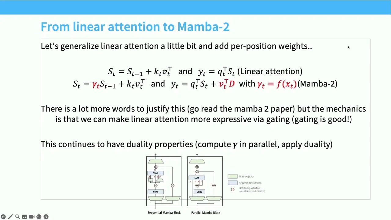
The recording ends mid-answer, around (59:30), with a question about linear attention versus sliding windows. He sketches it: instead of storing a cache, keep a compressed summary of history — the naive version sums key-value pairs into a single vector, giving you sequence-length independence by construction — and then gestures at Gated DeltaNet and Mamba as the more sophisticated versions. And that's where the file stops.
 

Where the Lecture Felt Unsettled

 

A few things I'd flag before you treat this as complete.
 

The roadmap he gives around (8:30) promises arithmetic intensity, KV cache reduction, quantization, pruning, speculative decoding, and practical concerns. The transcript ends at 59:58 mid-sentence. Quantization, pruning, and speculative decoding never arrive, and neither does the continuous batching he references at (28:30) as the fix for unpredictable concurrency. If there's a second recording or a follow-up session, that's where the rest lives.
 

The symbolic-to-numeric jump in the Llama example is the part I'd most want to rewatch. The intensity derivations are done symbolically on the board, then instantiated into concrete model numbers quite quickly, and I lost the thread on which terms were being kept. The per-sequence KV figure — something around 838 million, multiplying by B — was delivered at speed and I'm inferring the units. A spreadsheet alongside the slides would fix this.
 

The GQA-versus-MLA contradiction is presented honestly and then left unresolved, which is probably correct but leaves you without a decision rule for picking between them. His broader advice — distrust anything that isn't math — is good epistemics and unhelpful as an engineering heuristic. I found myself wanting the class after this one.
 

One small oddity: early on he describes GPT-4 as having come out earlier this year, which doesn't match any timeline I know. I'm filing that as a slip of the tongue rather than a claim, but don't build anything on it.
 

And the structural gap I keep coming back to: batch size during generation is treated as a variable you can choose, but for a live serving system it's a property of your traffic. He says continuous batching addresses it and then, in this recording, doesn't get there. That's the seam between the clean analysis and the messy deployment reality.
 

If you take one thing from the hour, take the asymmetry. Inference isn't training run backwards — it's a sequential, memory-bound problem where the thing you're optimizing (bytes moved per request) behaves nothing like the thing you optimized during pretraining, and where the metrics you'd naively treat as one thing split into a genuine fork between latency and throughput. Once you see generation as a stack of thin matmuls each dragging its own private KV cache, every technique in the second half stops looking like a bag of tricks and starts looking like the same idea applied at different angles.
 

Content Disclaimer:

This article is for general reference only and does not constitute professional R&D guidance, production process advice or quality certification. All material performance data has specific test premises; readers should verify parameters against actual equipment and working conditions.