Stanford CS329A Self‑Improving AI Agents ｜ Part 2 ｜ Test‑Time Compute Scaling — Annotated Lecture Notes & Key Takeaways

Course Information

Institution: Stanford

Original Course: Stanford CS329A Self‑Improving AI Agents ｜ Part 2 ｜ Test‑Time Compute Scaling

Instructor Bio: This session is co-instructed by **Aakanksha Chowdhery** and **Azalia Mirhoseini**, faculty and researchers at Stanford University and Google DeepMind. Aakanksha Chowdhery earned her PhD from Stanford University and is a Senior Researcher at Google DeepMind. She led end-to-end training of the 540B PaLM model and drove pre-training and scaling efforts for multiple generations of Gemini MoE models. She has also contributed core components to PaLM-E, Med-PaLM, and the Pathways infrastructure that underpins Google’s large language model ecosystem, with deep expertise in dense and Mixture-of-Experts architectures and large-scale model training. Azalia Mirhoseini is an Assistant Professor of Computer Science at Stanford University and founder of the Scaling Intelligence Lab. She also serves as a Senior Staff Scientist at Google DeepMind and co-founded Ricursive Intelligence. Previously she held research roles at Google Brain and Anthropic, contributing to the development of the Claude and Gemini model families. Her pioneering work spans MoE architectures, test-time compute scaling, and deep reinforcement learning for chip design (AlphaChip), with a core research focus on recursive self-improving AI systems.

Course Description: This lecture examines test-time compute scaling as a paradigm for improving model performance without increasing parameter count. It covers repeated sampling strategies, inference-time search frameworks such as Archon, and evidence showing that optimal scaling of test-time compute can outperform scaling model parameters. It also analyzes landmark work including Large Language Monkeys, and discusses practical tradeoffs between inference latency, compute cost, and solution quality.

This lecture digs into test‑time compute scaling, an idea that completely shifts how we think about making large language models more capable. Historically, nearly all performance improvements for LLMs came from pre‑training and fine‑tuning. The speaker makes the case that we can unlock major gains without touching a model’s underlying weights. All we need to do is allocate extra computing resources while the model works through a user’s query. The session walks through practical workflows such as repeated parallel sampling, real‑world benchmark outcomes, major weaknesses in existing verification tools, different inference‑based improvement strategies, and Archon, an automated framework built to mix and match these approaches. Student questions and group discussion pop up frequently, and plenty of unresolved research problems come to light along the way.
 

Repeated Sampling: Drawing Out Correct Answers With Extra Attempts

 

The lecturer opens by outlining the three established stages of LLM development. Pre‑training eats up enormous GPU capacity over months of work, trained against trillions of text tokens. Fine‑tuning uses far less data and computational power by comparison. Inference describes the phase where end‑users actually interact with the finished model (00:17‑01:12). For a long time, people treated inference as something cheap and one‑and‑done. This lecture pushes back hard against that default mindset.
 

The discussion starts with findings from the “Large Language Monkeys” paper, built around the classic infinite‑monkey thought experiment. The core logic is pretty simple. Feed the exact same problem to the model over many separate runs, collect every distinct response it produces, then deploy some form of checker to pick out which output is factually correct (01:15‑02:02). You never alter model parameters. You just keep asking the same question repeatedly.
 

What makes this compelling is what benchmark testing shows. Smaller open‑source models like different Llama variants can outperform single‑shot outputs from large closed systems such as GPT‑4o. The base model itself does not grow smarter. It already holds the knowledge required to solve difficult problems, but often fails to land on the right answer on its very first try. Generating many separate responses helps pull those correct answers to the surface (02:04‑03:07).
 

This repeated‑sampling method transfers well across many different task categories. The lecturer references BBench, a benchmark set up to mimic real‑world software engineers editing code and writing patches. With DeepSeek‑V3, running up to one thousand sample outputs pushes performance above what Claude 3.5 achieves on coding tasks (03:20‑04:38). This works best when unit tests are available. Unit tests act as an automated checker. You can build a higher‑performing system entirely from an open‑source base model, using nothing more than extra compute spent during inference.
 

From there, the talk moves to test‑time scaling laws, drawing comparisons to pre‑training scaling laws covered in an earlier class. Pre‑training scaling lets us forecast test‑set loss based on how much data, compute power, and model parameters we pour into training. For inference‑time compute, we see a comparable, predictable power‑law pattern. Coverage — meaning the percentage of problems solved by at least one generated sample — follows this pattern as we crank up the number of parallel samples pulled from the model (04:48‑06:03).
 

This trend holds across an extremely wide range of model sizes. It appears for tiny 70‑million‑parameter models all the way up to 70‑billion‑parameter models, and it holds for multiple problem domains (06:08‑07:33).
 

I struggled to follow some of the mathematical reasoning in this section. For any single problem, the odds of getting at least one correct answer out of K samples follows a straightforward exponential formula built from pass@1, the single‑attempt success rate. But when you test across a full dataset with mixed‑difficulty questions, you observe power‑law scaling instead. The lecturer explains that to produce this power‑law pattern, your dataset needs a long tail of extremely hard problems (07:38‑09:40). Lots of questions are easy and get solved on the very first sample. A shrinking subset of hard questions have very low single‑attempt success rates. This broad spread of problem difficulty across the dataset creates the aggregate power‑law results we see in real testing (09:43‑11:21).
 

This shifts practical engineering priorities. Companies used to pour hundreds of millions into pre‑training, spend moderately on fine‑tuning, and try to keep every individual inference call as cheap as possible. Now we have a viable alternative: spend more compute during inference to raise model capability. This extra inference‑side compute can even run offline. You can set AI agents loose to work through a task, generating large volumes of tokens and iterating to lift answer quality, without forcing an end‑user to sit and wait for results (11:28‑12:20).
 

Verifiers and the Generation‑Verification Gap

 

Repeated sampling only delivers real value if you can reliably tell which outputs are actually right. Solid automated checking tools are non‑negotiable for this workflow (12:24‑12:42). Some subject areas make verification fairly straightforward. Formal proof‑checking software can validate individual steps in mathematical reasoning. Writing unit tests for code is frequently simpler than solving the original programming challenge. Human writers can craft these unit tests, which then serve as ground‑truth checkers (12:47‑13:30).
 

One neat in‑lab project shared focuses on generating CUDA kernels with AI. An LLM takes PyTorch source code and tries to rewrite it into lower‑level, hardware‑optimized CUDA code. You do not need human reviewers to judge correctness. You feed identical inputs into both the original PyTorch implementation and the newly‑generated CUDA code. Matching outputs mean the generated kernel works correctly. On the Kernel‑Bench benchmark, coverage keeps improving as you generate more candidate CUDA implementations (13:33‑15:13). This same equivalence‑check idea applies to many cross‑language code translation jobs.
 

But many problem spaces lack these built‑in, perfect checkers. This creates what the lecturer calls the generation‑verification gap. Even when the model regularly produces at least one correct answer somewhere among dozens or thousands of samples, your selection tool may fail to pick that winning candidate (15:16‑18:08).
 

Majority voting is one popular, low‑effort selection strategy. You look over all generated answers and pick whichever response appears most often. Plots shown in‑lecture demonstrate that majority voting plateaus really quickly, usually after 10‑50 samples. Its performance sits far below the theoretical coverage you would get with a perfect, “oracle” verifier. This gap becomes much wider on harder benchmarks such as MATH compared to the more approachable GSM8K math dataset. Reward models — LLMs fine‑tuned to score response quality — shrink part of this gap, but still leave meaningful room for improvement (16:11‑17:47).
 

Why does majority voting fall apart on the toughest problems? For many of these hard‑to‑solve questions, the correct solution might only pop up one, two or three times out of thousands of total samples. Right answers show up very rarely. Since voting works off frequency counts, these rare correct outputs get overlooked completely (18:12‑19:22). That leaves us with a genuine practical puzzle: how do you spot that rare correct answer buried inside a huge pile of mostly‑wrong outputs?
 

At this point, the lecture shifts to short small‑group discussion among students. Several promising research directions come up. One student suggests pairing retrieval‑augmented generation with test‑time compute to balance response speed and accuracy. Another wonders if you could run exploratory, information‑gathering prompting first before kicking off rounds of parallel sampling. A third student points out you do not always need definitive proof an answer is right. Sometimes it is easier just to reliably spot wrong answers and filter those out, using simulations or external tooling. Someone else brings up the idea of building large ensembles of separate verifier models, though the lecturer notes this approach carries heavy compute costs (19:25‑25:12). The lab has published a dataset on Hugging Face containing thousands of samples per problem, meant for researchers working to close this generation‑verification gap.
 

Parallel Sampling, Sequential Revision and Reward‑Guided Tree Search

 

Everything discussed so far centers on parallel sampling: creating many full, independent answers all at once. Test‑time scaling also includes a second major family of techniques: sequential revision. Rather than generating dozens of complete answers from scratch, you start with one initial solution and repeatedly rewrite, critique, and refine it. You prompt the model to examine its own output from fresh angles and keep tweaking until it feels ready to finalize a reply (27:00‑28:13). You can pull this off purely through prompt engineering, though modern reasoning‑focused models already show similar revision‑style behaviours internally.
 

Reward models fall into two distinct buckets. Outcome‑based reward models (ORM) look only at the finished final answer and assign a quality score. Process reward models (PRM) dig deeper. They evaluate each individual reasoning step along the way, instead of judging nothing but the end result. For a multi‑step math solution, every logical chunk of reasoning gets its own separate score (28:58‑30:02). PRMs score meaningful reasoning steps, not individual tokens. Human annotators label whether each reasoning move is good or flawed during model training.
 

Process reward models make beam‑search‑style tree‑search possible during inference. Imagine you have a fixed compute budget. At each reasoning step you generate several possible next moves. Your PRM scores every potential path. You hold onto only the highest‑scoring branches and expand those further, cutting away low‑quality paths before you waste tokens exploring them (30:05‑31:22). PRMs perform best on tasks they saw during fine‑tuning, but still generalize somewhat to unfamiliar problem types.
 

Researchers have tested mixing parallel sampling workflows with sequential revision. You can spin up multiple parallel draft answers, run iterative refinement on each separate draft, and then rely on reward models to select the best final output. Lots of hybrid combinations are possible, and this whole space remains active, unfinished research (33:20‑34:40).
 

One cited paper uses the PaLM model on math benchmarks, sorting problems into difficulty groups based on pass@1 single‑attempt performance. The work compares majority voting, ORM‑driven selection, PRM‑guided tree search, and different hybrid setups. For easy and medium‑difficulty questions, adding extra test‑time compute can deliver larger per‑token performance gains than investing resources into bigger pre‑trained base models. For the absolute hardest problems, however, scaling pre‑training and using larger models still delivers better results, even with generous inference‑compute budgets (34:43‑39:01).
 

This creates one of the core tensions laid out in the lecture. Smaller open‑source models become noticeably more capable when you throw extra inference compute at them. Even so, there is a clear ceiling. No amount of test‑time scaling can completely erase the gap against top‑tier heavily‑pre‑trained frontier models on the most difficult tasks. The lecturer also brings up a practical real‑world angle: not every team can afford massive pre‑training runs. Test‑time scaling gives groups without huge pre‑training budgets a realistic path to lift model performance, even if it cannot solve every ultra‑hard challenge (39:04‑41:08).
 

One part of this discussion felt under‑explained to me. The talk states that hard problems still favour larger pre‑trained models, but never really unpacks why exactly this happens. Is it missing factual knowledge? Is it fundamental reasoning limits that sampling cannot work around? The lecturer leaves this hanging as an open research question rather than offering a concrete mechanistic explanation.
 

More student questions follow. One attendee asks about hybrid tree‑search approaches that blend sequential revision and parallel branching. Another puts forward an intuitive hypothesis: easier problems have many valid reasoning paths toward success, so sequential refinement works well. Very hard problems offer almost no correct paths, meaning you need heavy parallel sampling just to stumble onto at least one working solution (41:12‑45:21).
 

Archon: Hunting for Good Inference‑Time Architecture Combinations

 

The final major topic is Archon, short for architecture research framework for inference‑time scaling. One of the course TAs is listed as a co‑author for this work. Archon tries to answer a concrete practical question: given a fixed inference compute budget, what combination of inference‑time operations will maximize answer correctness (45:48‑46:18)?
 

You can view test‑time scaling itself as an architecture‑search problem. Your inputs are target benchmarks, your total allowed inference call budget, and a pool of available LLMs. You get access to a toolkit of different inference‑time operations. Archon’s ITAS (inference‑time architecture search) optimizer figures out how to stack and chain these operations together. Its output is a complete multi‑step inference pipeline tuned for your given constraints (46:24‑48:08).
 

The lecturer walks through each core building‑block operation:

• Generation: Draw fresh responses from one or more LLMs. This forms the base component for parallel sampling workflows.
• Fusion: Feed multiple candidate answers back into an LLM prompt, asking it to synthesize all those separate outputs into a single, improved final response. This fits under sequential‑style update patterns. One surprising experimental takeaway: fusion can generate better outputs than simply picking the single best sample from your pool, even when you have access to a perfect oracle selector (48:43‑53:15).
• Critic: Prompt a model to point out strengths and weaknesses for a given candidate answer.
• Ranker: Ask a model to sort candidate outputs by quality to produce an ordered list.
• Unit‑test generation and evaluation: Mostly relevant for coding challenges. The model writes test specifications or runnable unit tests, then judges existing code candidates against those tests (54:59‑56:22).

 

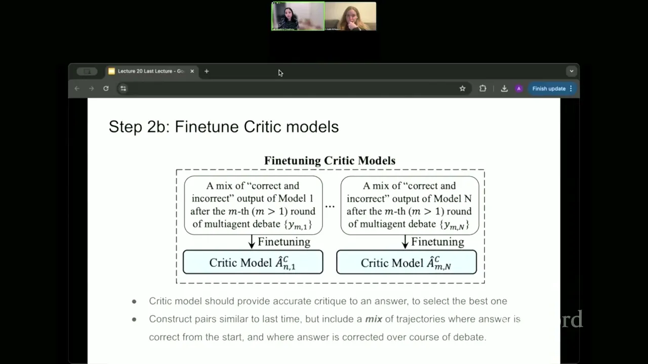
You can stack these operations across multiple layers. For coding‑focused pipelines, effective setups might first generate many code samples, create unit tests, run evaluations, then apply critics, rankers and fusion in repeated cascading stages. Running multiple stacked layers of these inference‑side operations improved accuracy in their testing. The effect draws loose parallels to stacking neural network layers during pre‑training (56:28‑59:29).
 

Searching through every single possible pipeline combination would burn through too many compute resources. Archon’s Bayesian optimizer narrows the search space by applying reasonable guardrails. Critics should run before rankers or fusion steps. Unit‑test generation must be immediately paired with unit‑test evaluation. It searches over pipeline setups against held‑out benchmark data, optimizing for accuracy while respecting limits on total inference calls (59:43‑1:01:21).
 

Archon can build pipelines tuned for one specific task, or more general‑purpose pipelines meant to perform reasonably well across many different benchmarks. In their reported results, pipelines built purely from open‑source models matched or beat closed‑source frontier models on pass@1 single‑answer quality for reasoning, math and coding benchmarks, with an average 14.1‑percent performance lift (1:01:24‑1:03:01).
 

The lecture ends by posing several thought‑provoking questions for students to work through on their own, as available class time runs out.
 

Test‑time compute scaling changes how we think about squeezing better performance from LLMs. We do not have to only chase ever‑larger pre‑trained models. We can instead spend extra compute while answering queries, using tools such as parallel sampling, iterative revision, reward‑guided tree‑search, and automated pipeline‑search systems like Archon. The biggest real‑world bottleneck remains building reliable verifiers, and the hardest problems still give an advantage to heavily pre‑trained large models.

Content Disclaimer: This article is for general reference only and does not constitute professional R&D guidance, production process advice or quality certification. All material performance data has specific test premises; readers should verify parameters against actual equipment and working conditions.